
The total costs of a company can be broken down into two parts: fixed costs and variable costs. Fixed costs do not vary with output (the number of units produced and sold), whereas variable costs vary with output.
Leverage is the use of fixed costs in a company’s cost structure. It has two components:
For highly leveraged firms, that is firms with a high proportion of fixed costs relative to total costs, a small change in sales will have a big impact on earnings.
Let’s look at an example to understand the impact of leverage.
Example
Consider two companies, HL and LL, with the same revenue and net income but a different cost structure.
| Operating Performance | Income Statement | ||||
| HL | LL | HL | LL | ||
| No. of units sold | 100 | 100 | Revenue | 100 | 100 |
| Sales price per unit | 1 | 1 | Operating costs | 70 | 75 |
| Variable cost per unit | 0.2 | 0.6 | Operating Income | 30 | 25 |
| Fixed operating cost | 50 | 15 | Financing Expense | 10 | 5 |
| Fixed financing cost | 10 | 5 | Net Income | 20 | 20 |
How is the cost structure different?
What is the impact on net income if sales numbers change?
Solution:
| Net income for different units of sold | ||||||
| HL | LL | HL | LL | HL | LL | |
| No. of units sold | 100 | 100 | 0 | 0 | 120 | 120 |
| Fixed operating costs | 50 | 15 | 50 | 15 | 50 | 15 |
| Variable costs | 20 | 60 | 0 | 0 | 24 | 72 |
| Operating costs | 70 | 75 | 50 | 15 | 74 | 87 |
| Operating Income | 30 | 25 | -50 | -15 | 46 | 33 |
| Interest expense | 10 | 5 | 10 | 5 | 10 | 5 |
| Net Income | 20 | 20 | -60 | -20 | 36 | 28 |
Let us plot the net income for different levels of sales (units sold) for HL and LL.
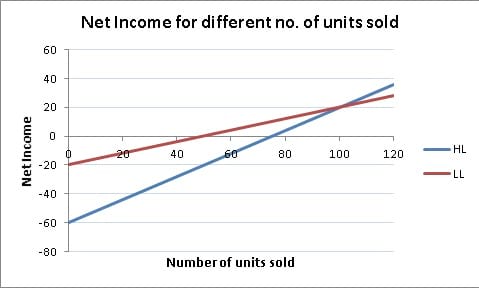
As you can see, the loss is magnified when revenue is zero and the profit is also magnified when revenue increases by a marginal amount for HL relative to LL. When 100 units are sold, the net income is the same for both the companies. The effect of both loss and profit is higher for a high leverage firm.
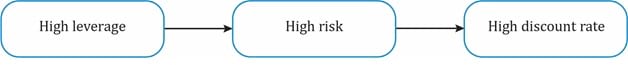
Leverage increases volatility of a company’s earnings and cash flows and also increases the risk of lending to or owning a company. The valuation of a company and its equity is affected by the degree of leverage. The higher a company’s leverage, the higher is its risk, which requires a higher discount rate to be applied in valuation.
Business risk is the risk associated with operating earnings. All firms face the risk that revenues will decline, which will in turn, affect operating earnings. Business risk consists of two components: sales risk and operating risk.
Business risk and its two components are depicted in the picture below:
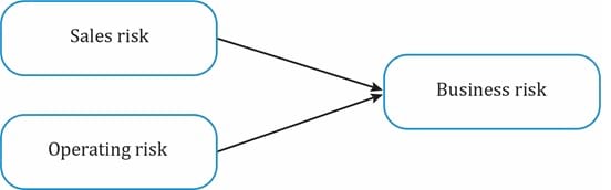
Sales risk is the variability in profits due to uncertainty of sales price and volume (product demand and revenue uncertainty).
Operating risk is the risk due to operating cost structure. It is greater when fixed operating costs are higher relative to variable operating costs.
Degree of operating leverage is a quantitative measure of operating risk. It is the ratio of the percentage change in operating income to the percentage change in units sold. It measures how sensitive a company’s operating income is to changes in sales. For example, a DOL of 2 means that a 1 percent change in units sold results in a 2 percent change in operating income.

It can be shown that DOL =
where:
Q = number of units
P = price per unit
V = variable operating cost per unit
F = fixed operating cost
P – V = per unit contribution margin
Q (P – V) = contribution margin
Example
Given the following data, compute DOL for HL and LL.
| HL | LL | |
| Number of units sold | 100 | 100 |
| Sales price per unit | 1 | 1 |
| Variable cost per unit | 0.2 | 0.6 |
| Fixed operating cost | 50 | 15 |
| Fixed financing cost | 10 | 5 |
Solution:
For HL:
Q = 100; P = 1; V = 0.2; F = 50
DOL for HL: = 2.67
For LL:
Q = 100; P = 1; V = 0.6; F = 15
DOL for LL: = 1.6
= 1.6
Financial risk is the risk associated with how a company finances its operations. A company may choose to finance using debt or equity. Greater the use of debt, greater is the company’s financial risk.
Degree of financial leverage is a quantitative measure of financial risk. For example, if DFL is 2, then a 5 percent increase in operating income will most likely result in a 10 percent increase in net income.
DFL =
It can be shown that DFL =
where
Q = number of units
P = price per unit
V = variable operating cost per unit
F = fixed operating cost
C = fixed financial cost
P-V = per unit contribution margin
Q (P – V) = contribution margin
Example
Given the following data, compute DFL for HL and LL.
| HL | LL | |
| Number of units sold | 100 | 100 |
| Sales price per unit | 1 | 1 |
| Variable cost per unit | 0.2 | 0.6 |
| Fixed operating cost | 50 | 15 |
| Fixed financing cost | 10 | 5 |
Solution:
For HL:
Q = 100; P = 1; V = 0.2; F = 50; C = 10
 = 1.5
= 1.5For LL:
Q = 100; P = 1; V = 0.6; F = 15; C = 5
 = 1.25
Effect of Financial Leverage on NI and ROE
Higher leverage leads to higher ROE volatility and potentially higher ROE levels. This is illustrated through a simple example. Consider two firms with the same operating income (EBIT), but different capital structures. While Firm 1 has no debt, capital structure of Firm 2 comprises 50% debt and 50% equity. The table below computes ROE for different levels of EBIT.
ROE = NI / equity
| Firm 1: Assets = 200; Equity = 200 Debt = 0; Tax = 0% | Firm 2: Assets = 200; Equity = 100; Debt = 100, Interest = 10% | |||
| EBIT | NI | ROE | NI | ROE |
| 0 | 0 | 0 | -10 | -10% |
| 20 | 20 | 10% | 10 | 10% |
| 40 | 40 | 20% | 30 | 30% |
| 60 | 60 | 30% | 50 | 50% |
| 80 | 80 | 40% | 70 | 70% |
Some inferences about the effect of financial leverage on NI and ROE:
Total leverage gives us the combined effect of both operating leverage and financial leverage. Degree of total leverage (DTL) measures the sensitivity of net income to changes in the number of units produced and sold.


where
Q = number of units
P = price per unit
V = variable operating cost per unit
F = fixed operating cost
C = fixed financial cost
P-V = per unit contribution margin
Q (P – V) = contribution margin
Example
Given the following data, compute DTL for HL and LL.
| HL | LL | |
| Number of units sold | 100 | 100 |
| Sales price per unit | 1 | 1 |
| Variable cost per unit | 0.2 | 0.6 |
| Fixed operating cost | 50 | 15 |
| Fixed financing cost | 10 | 5 |
Solution:
For HL:
Q = 100; P = 1; V = 0.2; F = 50; C = 10
 = 4
= 4For LL:
Q = 100; P = 1; V = 0.6; F = 15; C = 5
 = 2
= 2Breakeven point
Breakeven point is the number of units produced and sold at which net income is zero, the point at which revenues are equal to costs.
Breakeven point QBE =
where:
F = fixed operating costs
C = fixed financial cost
V = variable cost per unit
P = the price per unit
Operating breakeven point
Operating breakeven point is the number of units produced and sold at which operating income is zero.

All else equal companies that have high operating and financial leverage will have high break even points as compared to companies with low leverage. This is demonstrated in the following example.
The further away unit sales are from the breakeven point for high leverage companies, the greater the magnifying effect of this leverage.
Example
Given the following data, compute the breakeven and operating breakeven points for HL (high leverage) and LL (low leverage) companies.
| HL | LL | |
| Number of units sold | 100 | 100 |
| Sales price per unit | 1 | 1 |
| Variable cost per unit | 0.2 | 0.6 |
| Fixed operating cost | 50 | 15 |
| Fixed financing cost | 10 | 5 |
Solution:
For HL:
F = 50; C = 10; P = 1; V = 0.2
 = 75
= 75 = 50/0.8 = 62.5
For LL:
F = 15; C = 5; P = 1; V = 0.6
 = 50
= 50 = 15/0.4 = 37.5
Instructor’s Note: Section 8 ‘The Risks of Creditors and Owners’ is not testable and hence not covered.


Ace the Exam with Active Learning!

Ace the Exam with IFT Notes!

Practice your way to success!

Accelerate your studies!
 Do IFT Mocks to make you exam-ready!


Sign up to get more!