Exact matches only

Search in title

Search in content

Filter by Categories

101 concepts level I

101 concepts level II

2021 Level I Corporate Finance Full Videos

2021 Level I Economics Full Videos

2021 Level I Ethics Full Videos

2021 Level I FRA Full Videos

2021 Level I Portfolio Management Full Videos

2021 Level I Quantitative Methods Full Videos

Advice and How to Study Videos

All-Levels

Alternative Investments

Alternative Investments (AI)

BookLet Top Level

Corporate Issuers

Corporate Issuers (CI)

Demystified Videos

Derivatives

Derivatives (DV)

Economics

Economics (EC)

Equity

Equity Investments (EI)

Ethical and Professional Standards (ES)

Ethics

featured

Financial Reporting and Analysis

Financial Statement Analysis (FSA)

Fixed Income

Fixed Income (FI)

Level I

Level II

Level III

LM01 Alternative Investment Features, Methods, and Structures

LM01 Categories, Characteristics, and Compensation Structures of Alternative Investments

LM01 Corporate Structures and Ownership

LM01 Derivative Instrument and Derivative Market Features

LM01 Ethics and Trust in the Investment Profession

LM01 Fixed-Income Instrument Features

LM01 Fixed-Income Securities: Defining Elements

LM01 Introduction to Financial Statement Analysis

LM01 Market Organization & Structure

LM01 Market Organization and Structure

LM01 Organizational Forms, Corporate Issuer Features, and Ownership

LM01 Portfolio Management Overview

LM01 Portfolio Management: An Overview

LM01 Rates and Returns

LM01 The Firm & Market Structures

LM01 Time Value of Money

LM01 Topics in Demand and Supply Analysis

LM02 Alternative Investment Performance and Returns

LM02 Analyzing Income Statements

LM02 Code of Ethics and Standards of Professional Conduct

LM02 Code of Ethics and Standards of Professional Conduct Profession

LM02 Financial Reporting Standards

LM02 Fixed Income Markets - Issuance Trading and Funding

LM02 Fixed-Income Cash Flows and Types

LM02 Forward Commitment and Contingent Claim Features and Instruments

LM02 Introduction to Corporate Governance and Other ESG Considerations

LM02 Investors and Other Stakeholders

LM02 Organizing, Visualizing, and Describing Data

LM02 Performance Calculation and Appraisal of Alternative Investments

LM02 Portfolio Risk & Return: Part I

LM02 Portfolio Risk and Return Part I

LM02 Security Market Indexes

LM02 The Firm and Market Structures

LM02 Time Value of Money in Finance

LM02 Understanding Business Cycles

LM03 Aggregate Output, Prices and Economic Growth

LM03 Analyzing Balance Sheets

LM03 Business Models & Risks

LM03 Corporate Governance: Conflicts, Mechanisms, Risks, and Benefits

LM03 Derivative Benefits, Risks, and Issuer and Investor Uses

LM03 Fiscal Policy

LM03 Fixed-Income Issuance and Trading

LM03 Guidance for Standards I-VII

LM03 Guidance for Standards I–VII

LM03 Introduction to Fixed Income Valuation

LM03 Investments in Private Capital: Equity and Debt

LM03 Market Efficiency

LM03 Portfolio Risk & Return: Part II

LM03 Portfolio Risk and Return Part II

LM03 Private Capital, Real Estate, Infrastructure, Natural Resources, and Hedge Funds

LM03 Probability Concepts

LM03 Statistical Measures of Asset Returns

LM03 Understanding Income Statements

LM04 An Introduction to Asset-Backed Securities

LM04 Analyzing Statements of Cash Flows I

LM04 Arbitrage, Replication, and the Cost of Carry in Pricing Derivatives

LM04 Basics of Portfolio Planning & Construction

LM04 Basics of Portfolio Planning and Construction

LM04 Capital Investments

LM04 Common Probability Distributions

LM04 Fixed-Income Markets for Corporate Issuers

LM04 Introduction to the Global Investment Performance Standards (GIPS)

LM04 Monetary Policy

LM04 Overview of Equity Securities

LM04 Probability Trees and Conditional Expectations

LM04 Real Estate and Infrastructure

LM04 Understanding Balance Sheets

LM04 Understanding Business Cycles

LM04 Working Capital and Liquidity.

LM05 Analyzing Statements of Cash Flows II

LM05 Capital Investments and Capital Allocation

LM05 Company Analysis: Past and Present

LM05 Fixed-Income Markets for Government Issuers

LM05 Introduction to Geopolitics

LM05 Introduction to Industry and Company Analysis

LM05 Monetary and Fiscal Policy

LM05 Natural Resources

LM05 Portfolio Mathematics

LM05 Pricing and Valuation of Forward Contracts and for an Underlying with Varying Maturities

LM05 Pricing and Valuation of Forward Contracts.

LM05 Sampling and Estimation

LM05 The Behavioral Biases of Individuals

LM05 Understanding Cash Flow Statements

LM05 Understanding Fixed-Income Risk and Return

LM05 Working Capital & Liquidity

LM06 Analysis of Inventories

LM06 Capital Structure

LM06 Cost of Capital-Foundational Topics

LM06 Equity Valuation: Concepts and Basic Tools

LM06 Financial Analysis Techniques

LM06 Fixed-Income Bond Valuation: Prices and Yields

LM06 Fundamentals of Credit Analysis

LM06 Hedge Funds

LM06 Hypothesis Testing

LM06 Industry and Competitive Analysis

LM06 International Trade

LM06 Introduction to Geopolitics

LM06 Introduction to Risk Management

LM06 Pricing and Valuation of Futures Contracts

LM06 Simulation Methods

LM07 Analysis of Long-Term Assets

LM07 Business Models

LM07 Capital Flows and the FX Market

LM07 Capital Structure

LM07 Company Analysis: Forecasting

LM07 Estimation and Inference

LM07 International Trade and Capital Flows

LM07 Introduction to Digital Assets

LM07 Introduction to Linear Regression

LM07 Inventories

LM07 Pricing and Valuation of Interest Rate and Other Swaps

LM07 Pricing and Valuation of Interest Rates and Other Swaps

LM07 Technical Analysis

LM07 Yield and Yield Spread Measures for Fixed-Rate Bonds.

LM08 Currency Exchange Rates

LM08 Equity Valuation: Concepts and Basic Tools

LM08 Exchange Rate Calculations

LM08 Fintech in Investment Management

LM08 Hypothesis Testing

LM08 Long Lived Assets

LM08 Measures of Leverage

LM08 Pricing and Valuation of Options

LM08 Topics in Long-Term Liabilities and Equity

LM08 Yield and Yield Spread Measures for Floating-Rate Instruments

LM09 Analysis of Income Taxes

LM09 Income Taxes

LM09 Option Replication Using Put-Call Parity

LM09 Option Replication Using Put–Call Parity

LM09 Parametric and Non-Parametric Tests of Independence

LM09 The Term Structure of Interest Rates: Spot, Par, and Forward Curves

LM10 Financial Reporting Quality

LM10 Interest Rate Risk and Return

LM10 Non-current (Long-Term) Liabilities

LM10 Simple Linear Regression

LM10 Valuing a Derivative Using a One-Period Binomial Model

LM11 Financial Analysis Techniques

LM11 Financial Reporting Quality

LM11 Introduction to Big Data Techniques

LM11 Yield-Based Bond Duration Measures and Properties

LM12 Applications of Financial Statement Analysis

LM12 Introduction to Financial Statement Modeling

LM12 Yield-Based Bond Convexity and Portfolio Properties

LM13 Curve-Based and Empirical Fixed-Income Risk Measures

LM14 Credit Risk

LM15 Credit Analysis for Government Issuers

LM16 Credit Analysis for Corporate Issuers

LM17 Fixed-Income Securitization

LM18 Asset-Backed Security (ABS) Instrument and Market Features

LM19 Mortgage-Backed Security (MBS) Instrument and Market Features

New Booklet Top level

Portfolio Management

Portfolio Management (PM)

Quantitative Methods

Quantitative Methods (QM)

Uncategorized

Please select your exam.

IFT Notes for Level I CFA^® Program

LM10 Valuing a Derivative Using a One-Period Binomial Model

Part 1

1. Introduction

This learning module covers:

How to value a derivative using a one-period binomial model
The concept of risk-neutrality in derivatives pricing

2. Binomial Valuation

According to the law of one price, if the payoffs from any two assets at a given future date are identical, then the value of these two assets must also be identical today.

Forward commitments can be priced without making assumptions about the future price of the underlying asset. However, due to their asymmetric payoffs, the pricing of options requires a model to factor in the random price behavior of the underlying asset.

A commonly used model to determine the no-arbitrage value of an option is the binomial model.

3. The Binomial Model

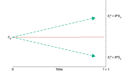
The binomial model assumes that over a given time period, there are only two possible outcomes – the asset’s price will either go up to $S_1^u$ or down to $S_1^d$ .
Let q denote the probability of an upward price movement and 1 – q denote the probability of a downward price movement. With only two possible outcomes, the sum of these two probabilities must equal to 1.
To value options, knowing q is not required, only the values $S_1^u$ and $S_1^d$ are needed. The difference between $S_1^u$ and $S_1^d$ represents the spread of possible future price outcomes or the volatility of the underlying asset.
We can also define the upward and downward moves in terms of returns
$R^u = \frac{S_1^u}{S_0>1}$
$R^d = \frac{S_1^d}{S_0<1}$

Exhibit 1 from the curriculum, illustrates the binomial model.

4. Pricing a European Call Option

Consider a one-year European call option with an exercise price (X) of 100.

The underlying spot price (S₀) is 80.

The two possible stock prices after 1 year are: $S_1^d$ = 60 and $S_1^u$ =110

We can compute the up and down returns as:
R^u = 110/80 = 1.375
R^d = 60/80 = 0.75

At t = 0, the call option value is c0.
At t = 1, the call option value is either $c_1^u$ (if the price goes up) or $c_1^d$ (if the price goes down). We can compute the values $c_1^u$ and $c_1^d$ as:

Up move: The call option ends in-the-money

$c_1^u=Max (0,S_T-X)=Max(0,110-100)=10$

Down move: The call option ends out-of-the-money

$c_1^d=Max (0,S_T-X)=Max(0,60-100)=0$

To compute c0 we can use replication and no-arbitrage pricing. Assume that at t = 0 we sell the call option at a price of c0 and purchase h units of the underlying asset. V0 represents the initial investment in the portfolio, and $V_1^u$ and $V_1^d$ represent the portfolio value if the underlying price moves up or down, respectively.

$V_0=hS_0-c_0$
$V_1^u=hS_1^u-c_1^u$
$V_1^d=hS_1^d-c_1^d$
We solve for h, such that the portfolio payoff in both the up and down scenarios are equal, i.e.:
$V_1^u=V_1^d$
$hS_1^u-c_1^u= hS_1^d-c_1^d$
Solving for h, we get:
$h=\frac{(c_1^u-c_1^d)}{(S_1^u-S_1^d )}$
This equation gives us the hedge ratio, or the proportion of the underlying that will offset the risk associated with an option.
The hedge ratio for our example is:
h= $\frac{(c_1^u-c_1^d)}{(S_1^u-S_1^d )}=(10-0)/(110-60)=0.20$
i.e. for each call option unit sold, we must buy 0.2 units of the underlying asset.
The portfolio values at t=1 for the up and down scenarios are:
$V_1^u=hS_1^u-c_1^u=0.20×110-10=12$
$V_1^d=hS_1^d-c_1^d=0.20×60-0=12$
As expected, the portfolio values are the same, which has two implications:
We can use either portfolio to value the derivative, and
The return $V_1^u/V_0=V_1^d/V_0$ must equal one plus the risk-free rate.

To prevent arbitrage, the portfolio value at t =1 should be discounted at the risk-free rate so that:
$V_0= \frac{V_1}{(1+r)}$
For our example, V1 =12. Assume that the annual risk-free rate is 5%. Therefore,
$V_0= \frac{12}{1.05}=11.42$
Replacing V0 by the hedged portfolio we get:
$hS_0-c_0=11.42$
$c_0=hS_0-11.42=0.2×80-11.42=4.58$
The value of the call option at t = 0 is 4.58.

Example:

(This is based on Example 1 from the curriculum.)

Hightest Capital believes that a particular non-dividend-paying stock is currently trading at $50 and is considering the sale of a one-year European call option at an exercise price of $55.

If the stock price is expected to either go up or down by 20% over the next year, what price should Hightest expect to receive for the sold call option? Assume a risk-free rate of 5%.

Solution:

S₀ = 50

$S_1^u=R^u S_0=1.2×50=60$
$S_1^d=R^d S_0=0.8×50=40$
The value of the call option at expiry is:
$c_1^u=Max (0,S_T-X)=Max(0,60-55)=5$
$c_1^d=Max (0,S_T-X)=Max(0,40-55)=0$

The hedge ratio of the option is:
$h=\frac{(c_1^u-c_1^d)}{(S_1^u-S_1^d )}= \frac{(5-0)}{(60-40)}=0.25$

The value of the hedged portfolio at maturity is:
$V_1=V_1^u=hS_1^u-c_1^u=0.25×60-5=10$

The present value of the hedged position today is:

V₀ = V₁(1 + r)⁻¹ = $10.00 × 1.05⁻¹ = 9.52

The call option value is:

c₀ = h*S₀ − V₀ = 0.25 × 50.00 − 9.52 = 2.98

5. Risk Neutrality

As seen in the previous section, neither the actual (real-world) probabilities of underlying price increases or decreases nor the expected return of the underlying are required to price an option. Only the expected volatility i.e. the values S_1^u and S_1^d are required to price an option.
Another method of calculating the value of a call option today, c0, is as the expected value of the option at expiration, c_1^u and c_1^d, discounted at the risk-free rate, r.

$c_0=\frac{({\pi} c_1^u+(1-{\pi}) c_1^d)}{(1+r)}^T$

In this equation π and (1-π) represent risk-neutral probabilities (rather than actual probabilities) of an up move and down move respectively.

The risk-neutral probability can be calculated as:

π= $\frac{(1+r-R^d)}{(R^u-R^d )}$

Substituting the details from our earlier example: Ru = 1.375, Rd = 0.75, $c_1^u$ = 10, $c_1^d$ =0 and assuming an annual risk-free rate of 5%, we get:
π= $\frac{(1+r-R^d)}{(R^u-R^d )}= \frac{(1+0.05-0.75)}{(1.375-0.75)}=0.48$
We can compute the value of c0 as:
$c_0=\frac{({\pi}c_1^u+(1-{\pi}) c_1^d)}{(1+r)^T} = \frac{(0.48×10+0.52×0)}{1.05}=4.57$
This matches our result from the previous section.

The risk-neutral probabilities used in this method are determined solely by the up and down gross returns, R^u and R^d, representing underlying asset volatility and the risk-free rate. The investor view on risk is not considered hence this method is referred to as risk-neutral pricing.

Example:

(This is based on Example 2 from the curriculum.)

Using the same details as Example 1:

“Hightest Capital believes that a particular non-dividend-paying stock is currently trading at $50 and is considering the sale of a one-year European call option at an exercise price of $55.

If the stock price is expected to either go up or down by 20% over the next year, what price should Hightest expect to receive for the sold call option? Assume a risk-free rate of 5%.”

Compute the risk-neutral probability of an up move and down move.
Calculate the no-arbitrage price of the call option.

Solution to 1:

The risk neutral probability of an up move is:
π= $\frac{(1+r-R^d)}{(R^u-R^d )}= \frac{(1+0.05-0.8)}{(1.2-0.8)}=0.625$
The risk-neutral probability of a down move is therefore:
1 – π = 1 – 0.625 = 0.375.