LM02 Portfolio Risk and Return Part I

Part 4

15. Efficient Frontier: Investment Opportunity Set & Minimum Variance Portfolios

15.1 Investment Opportunity Set

Consider the universe of risky, investable assets available to an investor. These can be combined to form many portfolios. When plotted together they form a curve. This set of portfolios is called the investment opportunity set as shown in the exhibit below.

15.2 Minimum Variance Portfolios  

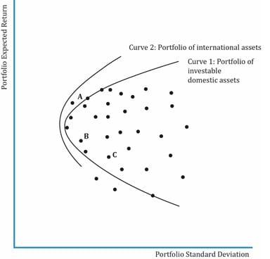
At any given level of return in the investment opportunity set, there will be a portfolio with minimum variance, i.e., minimum risk for a given level of return. The line combining such portfolios with minimum variance is called the minimum-variance frontier.

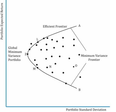
In the exhibit above, points M, N and O have the same expected return. But, investors will prefer point M over N or O because it has lower risk. The curve stretching from A to B through Z is called the minimum-variance frontier.

Global Minimum-Variance Portfolio: the portfolio with the lowest risk or minimum variance among portfolios of all risky assets is called the global minimum-variance portfolio. It is represented by point Z in the exhibit above. It is not possible to hold a portfolio of risky assets that has less risk than that of the global minimum-variance portfolio.

The efficient frontier is the part of the minimum variance frontier that is above the global minimum-variance portfolio. It represents the set of portfolios that will give the highest return at each risk level. Remember that the efficient frontier consists of only risky assets. There is no risk-free asset. Consider points L and M on the minimum-variance frontier. Both the portfolios have the same level of risk but portfolio L has a higher return than M. Investors will prefer the portfolio with higher return.

16. Efficient Frontier: A Risk-Free Asset and Many Risky Assets

One of the constraints of the efficient frontier is that it comprises only risky assets. We overcome this drawback with the capital allocation line: a combination of risky assets and a risk-free asset. The addition of a risk-free asset makes the investment opportunity set much richer than the investment opportunity set consisting only of risky assets. A portfolio of risky assets and a risk-free asset results in a straight line represented by the capital allocation line.

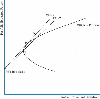
Interpretation of the diagram:

• CAL-P and CAL-Z are capital allocation lines formed by combining risky portfolios P and Z with the risk-free asset respectively.
• Portfolio P is the optimal risky portfolio. It is the point at which the capital allocation line is tangential to the efficient frontier of risky assets. CAL-P is the optimal capital allocation line.
• The optimal risky portfolio is based on the market and not the investor’s risk preferences. Along CAL-P, the weight of risk-free assets and portfolio P varies. For instance, it is 100% in the risk-free asset at y-axis, 100% in risky portfolio P at the point P, and a mix of both in between.

17. Efficient Frontier: Optimal Investor Portfolio

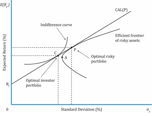
To identify the optimal investor portfolio, we must consider the investor’s risk preferences. The utility of each investor is best represented by his indifference curves. The optimal investor portfolio is the point at which the investor’s indifference curve is tangential to the optimal allocation line. Portfolio C in the exhibit below is the optimal investor portfolio.

Share on :