Exact matches only

Search in title

Search in content

Filter by Categories

101 concepts level I

101 concepts level II

2021 Level I Corporate Finance Full Videos

2021 Level I Economics Full Videos

2021 Level I Ethics Full Videos

2021 Level I FRA Full Videos

2021 Level I Portfolio Management Full Videos

2021 Level I Quantitative Methods Full Videos

Advice and How to Study Videos

All-Levels

Alternative Investments

Alternative Investments (AI)

BookLet Top Level

Corporate Issuers

Corporate Issuers (CI)

Demystified Videos

Derivatives

Derivatives (DV)

Economics

Economics (EC)

Equity

Equity Investments (EI)

Ethical and Professional Standards (ES)

Ethics

featured

Financial Reporting and Analysis

Financial Statement Analysis (FSA)

Fixed Income

Fixed Income (FI)

Level I

Level II

Level III

LM01 Alternative Investment Features, Methods, and Structures.

LM01 Categories, Characteristics, and Compensation Structures of Alternative Investments

LM01 Corporate Structures and Ownership

LM01 Derivative Instrument and Derivative Market Features

LM01 Derivative Instrument and Derivative Market Features.

LM01 Ethics and Trust in the Investment Profession

LM01 Ethics and Trust in the Investment Profession.

LM01 Fixed-Income Instrument Features.

LM01 Fixed-Income Securities: Defining Elements

LM01 Introduction to Financial Statement Analysis

LM01 Introduction to Financial Statement Analysis.

LM01 Market Organization & Structure.

LM01 Market Organization and Structure

LM01 Organizational Forms, Corporate Issuer Features, and Ownership.

LM01 Portfolio Management Overview

LM01 Portfolio Management: An Overview.

LM01 Rates and Returns.

LM01 The Firm & Market Structures.

LM01 Time Value of Money

LM01 Topics in Demand and Supply Analysis

LM02 Alternative Investment Performance and Returns.

LM02 Analyzing Income Statements.

LM02 Code of Ethics and Standards of Professional Conduct Profession

LM02 Code of Ethics and Standards of Professional Conduct.

LM02 Financial Reporting Standards

LM02 Fixed Income Markets - Issuance Trading and Funding

LM02 Fixed-Income Cash Flows and Types.

LM02 Forward Commitment and Contingent Claim Features and Instruments

LM02 Forward Commitment and Contingent Claim Features and Instruments.

LM02 Introduction to Corporate Governance and Other ESG Considerations

LM02 Investors and Other Stakeholders.

LM02 Organizing, Visualizing, and Describing Data

LM02 Performance Calculation and Appraisal of Alternative Investments

LM02 Portfolio Risk & Return: Part I.

LM02 Portfolio Risk and Return Part I

LM02 Security Market Indexes

LM02 Security Market Indexes.

LM02 The Firm and Market Structures

LM02 Time Value of Money in Finance.

LM02 Understanding Business Cycles.

LM03 Aggregate Output, Prices and Economic Growth

LM03 Analyzing Balance Sheets.

LM03 Business Models & Risks

LM03 Corporate Governance: Conflicts, Mechanisms, Risks, and Benefits.

LM03 Derivative Benefits, Risks, and Issuer and Investor Uses

LM03 Derivative Benefits, Risks, and Issuer and Investor Uses.

LM03 Fiscal Policy.

LM03 Fixed-Income Issuance and Trading.

LM03 Guidance for Standards I-VII

LM03 Guidance for Standards I–VII.

LM03 Introduction to Fixed Income Valuation

LM03 Investments in Private Capital: Equity and Debt.

LM03 Market Efficiency

LM03 Market Efficiency.

LM03 Portfolio Risk & Return: Part II.

LM03 Portfolio Risk and Return Part II

LM03 Private Capital, Real Estate, Infrastructure, Natural Resources, and Hedge Funds

LM03 Probability Concepts

LM03 Statistical Measures of Asset Returns.

LM03 Understanding Income Statements

LM04 An Introduction to Asset-Backed Securities

LM04 Analyzing Statements of Cash Flows I.

LM04 Arbitrage, Replication, and the Cost of Carry in Pricing Derivatives

LM04 Arbitrage, Replication, and the Cost of Carry in Pricing Derivatives.

LM04 Basics of Portfolio Planning & Construction

LM04 Basics of Portfolio Planning and Construction.

LM04 Capital Investments

LM04 Common Probability Distributions

LM04 Fixed-Income Markets for Corporate Issuers.

LM04 Introduction to the Global Investment Performance Standards (GIPS)

LM04 Introduction to the Global Investment Performance Standards (GIPS).

LM04 Monetary Policy.

LM04 Overview of Equity Securities

LM04 Overview of Equity Securities.

LM04 Probability Trees and Conditional Expectations.

LM04 Real Estate and Infrastructure.

LM04 Understanding Balance Sheets

LM04 Understanding Business Cycles

LM04 Working Capital and Liquidity.

LM05 Analyzing Statements of Cash Flows II.

LM05 Capital Investments and Capital Allocation.

LM05 Company Analysis: Past and Present.

LM05 Fixed-Income Markets for Government Issuers.

LM05 Introduction to Geopolitics.

LM05 Introduction to Industry and Company Analysis

LM05 Monetary and Fiscal Policy

LM05 Natural Resources.

LM05 Portfolio Mathematics.

LM05 Pricing and Valuation of Forward Contracts and for an Underlying with Varying Maturities

LM05 Pricing and Valuation of Forward Contracts.

LM05 Sampling and Estimation

LM05 The Behavioral Biases of Individuals

LM05 The Behavioral Biases of Individuals.

LM05 Understanding Cash Flow Statements

LM05 Understanding Fixed-Income Risk and Return

LM05 Working Capital & Liquidity

LM06 Analysis of Inventories.

LM06 Capital Structure.

LM06 Cost of Capital-Foundational Topics

LM06 Equity Valuation: Concepts and Basic Tools

LM06 Financial Analysis Techniques

LM06 Fixed-Income Bond Valuation: Prices and Yields.

LM06 Fundamentals of Credit Analysis

LM06 Hedge Funds.

LM06 Hypothesis Testing

LM06 Industry and Competitive Analysis.

LM06 International Trade.

LM06 Introduction to Geopolitics

LM06 Introduction to Risk Management

LM06 Introduction to Risk Management.

LM06 Pricing and Valuation of Futures Contracts

LM06 Pricing and Valuation of Futures Contracts.

LM06 Simulation Methods.

LM07 Analysis of Long-Term Assets.

LM07 Business Models.

LM07 Capital Flows and the FX Market.

LM07 Capital Structure

LM07 Company Analysis: Forecasting.

LM07 Estimation and Inference.

LM07 International Trade and Capital Flows

LM07 Introduction to Digital Assets.

LM07 Introduction to Linear Regression

LM07 Inventories

LM07 Pricing and Valuation of Interest Rate and Other Swaps.

LM07 Pricing and Valuation of Interest Rates and Other Swaps

LM07 Technical Analysis

LM07 Yield and Yield Spread Measures for Fixed-Rate Bonds.

LM08 Currency Exchange Rates

LM08 Equity Valuation: Concepts and Basic Tools.

LM08 Exchange Rate Calculations.

LM08 Fintech in Investment Management

LM08 Hypothesis Testing.

LM08 Long Lived Assets

LM08 Measures of Leverage

LM08 Pricing and Valuation of Options

LM08 Pricing and Valuation of Options.

LM08 Topics in Long-Term Liabilities and Equity.

LM08 Yield and Yield Spread Measures for Floating-Rate Instruments.

LM09 Analysis of Income Taxes.

LM09 Income Taxes

LM09 Option Replication Using Put-Call Parity

LM09 Option Replication Using Put–Call Parity.

LM09 Parametric and Non-Parametric Tests of Independence.

LM09 The Term Structure of Interest Rates: Spot, Par, and Forward Curves.

LM10 Financial Reporting Quality.

LM10 Interest Rate Risk and Return.

LM10 Non-current (Long-Term) Liabilities

LM10 Simple Linear Regression.

LM10 Valuing a Derivative Using a One-Period Binomial Model

LM10 Valuing a Derivative Using a One-Period Binomial Model.

LM11 Financial Analysis Techniques.

LM11 Financial Reporting Quality

LM11 Introduction to Big Data Techniques.

LM11 Yield-Based Bond Duration Measures and Properties.

LM12 Applications of Financial Statement Analysis

LM12 Introduction to Financial Statement Modeling.

LM12 Yield-Based Bond Convexity and Portfolio Properties.

LM13 Curve-Based and Empirical Fixed-Income Risk Measures.

LM14 Credit Risk.

LM15 Credit Analysis for Government Issuers.

LM16 Credit Analysis for Corporate Issuers.

LM17 Fixed-Income Securitization.

LM18 Asset-Backed Security (ABS) Instrument and Market Features.

LM19 Mortgage-Backed Security (MBS) Instrument and Market Features.

New Booklet Top level

Portfolio Management

Portfolio Management (PM)

Quantitative Methods

Quantitative Methods (QM)

Uncategorized

Please select your exam.

IFT Notes for Level I CFA^® Program

LM02 Portfolio Risk and Return Part I

Part 2

7. Historical Return and Risk

Historical return is the return actually earned in the past, while expected return is the return one expects to earn in the future.

Historical data shows that higher returns were earned in the past by assets with higher risk. Of the three major asset classes in the U.S., namely stocks, bonds, and T-bills, it has been observed that stocks had the highest risk and return followed by bonds, and T-bills had the lowest return and lowest risk.

Asset Class	Annual Average Return	Standard Deviation (Risk)
Small-cap stocks	High ↓ Low	High ↓ Low
Large-cap stocks
Long-term corporate bonds
Long-term treasury bonds
Treasury bills

8. Other Investment Characteristics

In evaluating investments using mean and variance, we make the following two assumptions:

Assumption 1: Distributional characteristics.
Returns are normally distributed. If this assumption does not hold, then consider skewness and kurtosis. These concepts have been covered earlier in quantitative methods.

Assumption 2: Market characteristics.
Markets are informationally and operationally efficient. If markets are not operationally efficient, then it leads to: 1) high transaction costs 2) wide bid-ask spreads and 3) larger price impact of trades.

9. Risk Aversion and Portfolio Selection & The Concept of Risk Aversion

9.1 The Concept of Risk Aversion

Risk aversion refers to the behavior of investors preferring less risk to more risk.

Risk tolerance is the amount of risk an investor is willing to take for an investment. High risk aversion is the same as low risk tolerance. Three types of risk profiles are outlined below:

Risk Seeking: A risk seeking investor prefers high return and high risk. Given two investments, A and B, where both have the same return but investment A has higher risk, he will prefer investment A.
Risk Neutral: A risk neutral investor is concerned only with returns, and is indifferent about the risk involved.
Risk Averse: A risk averse investor will prefer an investment that has lower risk, all else equal. Given two investments, A and B, where both have the same return but investment A has higher risk, he will prefer investment B.

10. Utility Theory and Indifference Curves

The utility of an investment can be calculated as:

Utility = E(r) – 0.5 x A x ?²

where:

A = measure of risk aversion (the marginal benefit expected by the investor in return for taking additional risk. A is higher for risk-averse individuals.

𝜎² = variance of the investment

E(r) = expected return

Instructor’s Note:

While using this formula, use only decimal values for all parameters.

Example

An investor with A = 2 owns a risk-free asset returning 5%. What is his utility?

Solution:

Utility = 0.05 – 0.5 x 2 x 0 = 0.05

Now, he is considering an asset with 𝜎 = 10%. At what level of return will he have the same utility?

0.05 = E(r) – 0.5 x 2 x 0.1². Solving for E(R) we get 0.06 or 6.00%.

Given a choice between a risk-free asset and stock with an expected return of 10% and 𝜎 = 20%, what will he prefer?

U = 0.1 – 0.5 * 2 * 0.2² = 0.06. Since the utility number of 0.06 is higher than 0.05, the investor will prefer this investment over the previous one.

Indifference Curves

The indifference curve is a graphical representation of the utility of an investment. An indifference curve plots various combinations of risk-return pairs that an investor would accept to maintain a given level of utility. If the combinations of risk-return on a curve provide the same level of utility, then the investor would be indifferent to choosing one. Each point on an indifference curve shows that the investor is indifferent to what investment he chooses (risk/return combination) as long as the utility is the same.

To understand the indifference curve, let us plot all these numbers – expected return, standard deviation, and utility – on a graph.

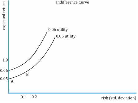
The key points to note are:

The indifference curves run from south-west to north-east. This is intuitive because for taking on higher risk (going east), investors expect to be compensated with higher expected return (going north).
The utility of points A and B are 0.05. This means that the investor will be indifferent about choosing an investment with E(r) of 5%, ? = 0 versus another with E(r) of 6%, ? = 10% as both have the same utility. Similarly, for assuming higher levels of risk, the investor is compensated with higher return as shown in the 0.05 utility curve. Along this curve, the investor is indifferent about choosing one point (investment) over the other.
As the investor moves north-west, he is happier as his utility increases, in this case from 0.05 to 0.06. Risk is compensated with higher returns and it signifies higher risk aversion.

We now consider the indifference curves for different types of investors.

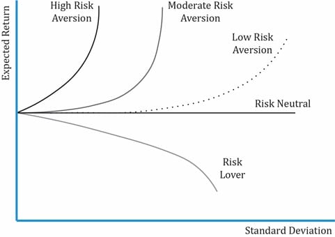
The exhibit above shows the indifference curves for different types of investors with expected return on y-axis and standard deviation on x-axis. Note the following:

Risk-neutral investor: For a risk-neutral investor, the utility is the same irrespective of risk as the investor is concerned only about the return. The expected return is constant.
Risk-averse investor: For a risk-averse investor, the curve is upward sloping, as the investor expects additional return for taking additional risk. Finance theory assumes that most investors are risk averse, but the degree of aversion may vary. The curve is steeper for investors with high risk-aversion.
Risk-seeking investor: The curve is downward sloping as the expected return decreases for higher levels of risk. It is not commonly seen.

11. Application of Utility Theory to Portfolio Selection

Now that we have seen utility theory and indifference curves for various investors, let us see how to apply it in portfolio selection. The simplest case is when a portfolio comprises two assets: a risk-free asset and a risky asset. For a high-risk averse investor, the choice is easy, to invest 100% in the risk-free asset but at the cost of lower returns. Similarly, for a risk-lover it would be to invest 100% in the risky asset. But is it the optimal allocation of assets, or can there be a trade-off?

Example

Consider a simple portfolio of a risk-free asset and a risky asset. Plot the expected return of the portfolio against the risk of the portfolio for different weights of the two assets.

Risk-free asset	Risky asset
R_f = 5%	R_i= 10%
? = 0	?_i= 20%

Solution:

A portfolio’s standard deviation is calculated as:

?_p= $\sqrt{w_1^2 * \sigma_1^2 + w_2^2 * \sigma_2^2 + 2 * w_1 * w_2 * \rho_{1,2} * \sigma_1 * \sigma_2}$

Given that ?₁ = 0, the terms $w_1^2 * \sigma_1^2 \text{and} 2 * w_1 * w_2 * \rho_{1,2} * \sigma_1 * \sigma_2$ become zero as the correlation between a risk-free asset with risky asset is zero.

So, the equation becomes ?_p = w_{2 *}?₂. For different weights of the risky asset, let’s calculate the values for risk and return and plot portfolio risk-return on a graph. Note that the expected return is a weighted average of the two assets.

Weight of risky asset = w₂	?_p(portfolio risk) = w₂* ?₂	*R_p(Portfolio return) = w₁ R_f + w₂ * R_i**
0	0	5%
0.25	5%	6.25%
0.5	10%	7.5%
1	20%	10%

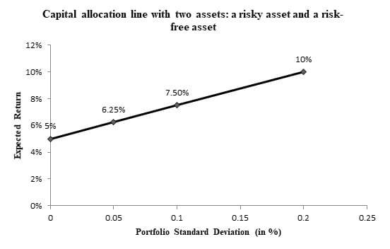
Graph interpretation:

What you get by plotting risk and return values for different weights of the risky and risk-free asset is a straight line (linear).
As you move north-east, the weight of the risky asset increases. The lowest point on the left corner, intersecting the y-axis with expected return of 5%, represents 100% in the risk-free asset. Similarly, the topmost point on the right corner represents 100% in the risky asset with expected return of 10%.
The straight line you see in the chart above is called the capital allocation line which represents the portfolios available to the investor as each point on the line is an investable portfolio.
So, how does an investor decide which portfolio to invest in? The answer is by combining an investor’s indifference curves and CAL to determine the optimal portfolio. We look at it in detail in the next section.

What is the Optimal Portfolio?
We get the optimal portfolio by combining the indifference curves and the capital allocation line. The utility theory gives us the indifference curves for an individual, while the capital allocation lines give us a set of feasible investments. The optimal portfolio for an investor will lie somewhere on the capital allocation line, i.e., some combination (weight) of the risky asset and risk-free asset. Using an investor’s risk-aversion measure A, we can use the utility theory to plot the indifference curves for an individual. Assume the indifference curves for this investor look as shown in the exhibit below:

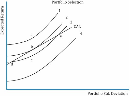
Some key points about the graph:

Curves 1, 2, 3, and 4 are various indifference curves for an individual. The indifference curves cannot intersect each other.
Curve 1 lies above the CAL. Curve 2 is tangential to the CAL at point b. Curve 3 intersects CAL at two points: d and e. Curve 4 lies below the CAL.
Curve 1 has the highest utility while Curve 4 has the lowest utility. As we discussed before, the investor is happier when we move north-west. Of the four curves, he will be happiest with curve 1. But, as curve 1 lies outside the CAL, it is not possible to construct a portfolio at any point on this curve with the available assets.
Points on curve 3 may be attainable with the two assets. To achieve the utility level of curve 3, the investor may choose to invest at points d and e where it intersects with CAL.
However, curve 2 is preferred over curve 3, as it provides a higher utility. To achieve this utility level, the investor may choose to invest at point b, where the indifference curve is tangential to the capital allocation line
This point, b, represents the optimal portfolio.

If another investor has a higher level of risk aversion, where will his optimal portfolio lie? With a higher risk aversion level, the indifference curves will be steeper. The tangential point will be closer to the risk-free asset, so it will be to the south-west of point b.