
Note: there is no explicit learning outcome associated with this section.
In this reading, we saw one return-generating model, the CAPM. But there are more models to estimate the return of an asset.
CAPM is popular because of its simplicity to estimate the expected return. However, there are several theoretical and practical limitations because of its unrealistic assumptions.
Theoretical limitations of the CAPM are as follows:
Practical limitations of the CAPM are as follows:
Other models are considered because of the limitations of CAPM. Of course these models, too, come with their own limitations. The models can be broadly categorized into theoretical and practical models.
Theoretical models
In principle, theoretical models are similar to the CAPM but with additional risk factors. One example is the arbitrage pricing theory (APT) which takes the following form:

where k is the number of risk factors, is the risk premium and
  is the sensitivity of the portfolio to factor k.
The drawback of this model is that it is difficult to identify risk factors and estimate sensitivity to each factor.
Practical Models
The Fama-French three-factor model and four-factor model have been found to predict asset returns better than the CAPM, which considers only beta risk. The three factors included in the Fama-French model are relative size, relative book-to-market value, and beta of the asset. The four-factor model adds one more momentum factor to the three-factor model. These models have limitations too. They cannot be applied to all assets and there is no certainty that these will work in the future.
Before selecting an investment manager, it is important for investors to understand the performance of a manager and the cost structure involved. In this section, we look at four measures that are commonly used in performance evaluation. These are:
| Sharpe Ratio |  = =  |
| M-Squared |  |
| Treynor Ratio |  = =  |
| Jensen’s Alpha | Actual portfolio return – expected return = ![R_p-[R_f+β(R_m-R_f )]](https://ift.world/wp-content/ql-cache/quicklatex.com-25e9ef8bf3c66ab2317d19d094f9620f_l3.png "Rendered by QuickLaTeX.com") |
Sharpe ratio is the excess return of the portfolio over the risk-free rate divided by the portfolio risk. It is the excess return per unit of risk. The higher the Sharpe ratio the better, all else equal. Sharpe ratio is the slope of the capital allocation line and represents the reward-to-variability ratio. The ex-ante and ex-post Sharpe ratio are given by:

→ evaluate the expected risk-adjusted return of the portfolio

→ to evaluate historical risk-adjusted returns.
Advantages of Sharpe ratio
Limitations of Sharpe ratio
Treynor ratio is the excess return of the portfolio over the risk-free rate divided by the systematic risk of the portfolio. The numerator must be positive for meaningful results. It does not work for negative beta assets.
The ex-ante and ex-post Treynor ratios are provided below.


Limitations of Treynor ratio
If M-Squared return (also known as risk adjusted performance measure or RAP) is greater than zero, the manager (portfolio) has positive risk-adjusted return. One way to get a positive M-Squared is when the risk is same as the market but RP is greater than RM. Another way is when the return is same as the market but at a lower risk. If M-Squared is zero, then the manager (portfolio) has the same risk-adjusted return as the market. If M-Squared return is negative, the manager (portfolio) has a lower risk-adjusted return than the market.
The ex-ante and ex-post M2 are given by:
![M^2=\left[E\left(R_p\right)-R_f\right]\frac{\sigma_m}{\sigma_p}+R_f=\mathrm{SR}\mathrm{\times }\sigma_m+R_f](https://ift.world/wp-content/ql-cache/quicklatex.com-6a15c8bb2439e5fa3844294f5f1d60c0_l3.png "Rendered by QuickLaTeX.com")
(ex ante)

(ex post)
where:  is the standard deviation of the market portfolio and
  is the portfolio-specific leverage ratio.
The difference between the risk-adjusted performance of the portfolio and the performance of the market is called M2 alpha.
Advantage: M-Squared is in units of the percent return which makes it more intuitive for the interpretation by the user.
Limitation: A limitation of this measure is that it uses total risk and not systematic risk.
Jensen’s alpha is the difference between the actual return on a portfolio and the CAPM calculated, expected or required return. In other words, it is the plot of the excess return of the security on the excess return of the market. The intercept is Jensen’s alpha and beta is the slope. Jensen’s alpha can be calculated on both ex ante and ex post basis.
Like the Treynor ratio, it is based on systematic risk. Alpha is used to rank different managers and their portfolios. Since Jensen’s alpha uses systematic risk, it is theoretically superior to M-Squared.
Interpreting Jensen’s Alpha
Instructor’s Note:
Sharpe ratio and M-squared are total risk measures. Use these measures when a portfolio is not fully diversified.
Treynor ratio and Jensen’s alpha are based on beta risk and should be used when a portfolio is well diversified.
12.1 Security Characteristic Line
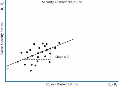
The SCL is a plot of the excess return of a security over the risk-free rate on the y-axis, against the excess return of the market on the x-axis. We saw earlier that the SML’s intercept on the y-axis is the alpha and the line’s slope is its beta. Similarly, the SCL’s slope is the security’s beta.
The SCL is obtained by regressing excess security return on the excess market return.

where:
 = excess security return
 = excess market return
 = Jensen’s alpha or excess return
In CAPM, we assumed that investors have homogeneous expectations and assign the same value to all assets. So all the investors arrive at the same optimal risky portfolio: the market portfolio. But, in reality, it does not actually happen.
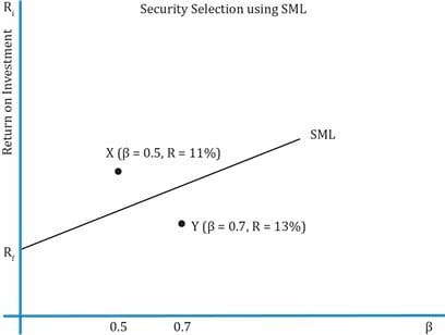
The SML can also be used for security selection. Investors can plot a security’s expected return and beta against the SML. The security is undervalued if it plots above the SML. The security is overvalued if it plots below the SML. The security is fairly priced if it plots on the SML.
As you can see in the exhibit below, security X is undervalued as it plots above the SML. At a risk level of β=0.5, the return of X is greater than the security that plots on the SML. Similarly, Y must not be bought because the security on SML at a risk level of β=0.7 has a higher return than Y.
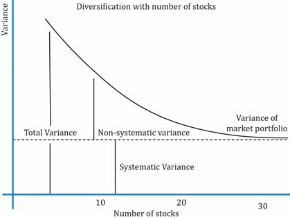
Theoretically, investors should hold a combination of the risk-free asset and the market portfolio but it is impractical to own the market portfolio as it has a large number of securities. For example, S&P 500 is a good representation of the market as it has 500 stocks. But it can be shown that holding as few as 30 stocks can diversify away the non-systematic risk.
Interpretation of the exhibit below:


Ace the Exam with Active Learning!

Ace the Exam with IFT Notes!

Accelerate your studies!

Practice your way to success!
 Do IFT Mocks to make you exam-ready!


Sign up to get more!