IFT Notes for Level I CFA^® Program

LM03 Portfolio Risk and Return Part II

Part 2

5. Systematic and Nonsystematic Risk

We have seen repeatedly that high returns come with high risk. But does all high risk lead to high returns? No. Total risk can be decomposed into systematic and nonsystematic risk.

Total variance = Systematic variance + Nonsystematic variance

5.1. Systematic Risk and Nonsystematic Risk

Systematic risk is non-diversifiable or market risk that affects the entire economy and cannot be diversified away. Investors get a return for systematic risk.

Examples of systematic risk are interest rates, inflation, natural disasters, unrest/coup attempts such as events in Middle East/Africa since 2011 and political uncertainty.

It is tough to avoid systematic risk. However, the effects can be minimized by selecting securities with low correlation to the rest of the portfolio.

Nonsystematic risk is a local risk that affects only a particular asset or industry. There is no compensation for nonsystematic risk as it can be diversified away.

Examples of nonsystematic risk are oil discoveries, non-approval for a drug, new regulations for telecom industry.

Nonsystematic risk may be avoided by diversifying a portfolio to include assets across countries, industries, and asset classes. Nonsystematic risk does not earn a return.

Pricing of risk: Pricing an asset is equivalent to estimating its expected rate of return; price and return are often used interchangeably. For example, if we know the cash flows for a bond, its price can be computed using the discount rate. Pricing of risk is this rate of return which reflects the systematic risk.

Instructor’s Note

Systematic risk or market risk is the only risk for which investors get compensated. It cannot be eliminated with diversification.

A risk-free asset has zero systematic risk and zero nonsystematic risk.

Example

Describe the systematic and nonsystematic risk components of the following assets:

A six-month Treasury bill.
An index fund based on the S&P 500, with a total risk of 18%.

Solution:

A six-month Treasury bill: For a T-bill, we know how much an investor would get paid at the end of six months. The systematic risk and nonsystematic risk are both zero; the total variance is therefore zero.
An index fund based on the S&P 500, with a total risk of 18%: S&P 500 represents the market. There is no nonsystematic risk in a market portfolio. So, the total risk of 18% is systematic risk.

Example

Consider two assets X and Y. X has a total risk of 25% of which 15% is systematic risk. Asset Y is the S&P index fund mentioned above with a total risk of 18%, all of which is systematic risk. Which asset will have a higher expected rate of return?

Solution:

Based on total risk, asset X seems an obvious choice because higher risk results in higher return. However it is more appropriate to compare the systematic risk of the two assets as only systematic risk earns a return. Asset Y will earn a higher expected return as its systematic risk of 18% is higher than asset X’s 15%. An investor will not be compensated for assuming nonsystematic risk in asset X as it can be eliminated.

6. Return-Generating Models

Return-generating models provide an estimate of the expected return of a security given certain input parameters called factors. If the model uses many factors, it is called a multi-factor model. If it uses one factor, it is a single-factor model.

Multi-factor Models

The three commonly used multi-factor models are: macroeconomic, fundamental, and statistical models. These models use factors that are correlated with security returns.

Macroeconomic models use economic factors such as economic growth, interest rate, unemployment rate, productivity, etc.
Fundamental models use input parameters such as earnings, earnings growth, cash flow, market capitalization, industry-specific inputs, financial ratios like P/E, P/B, value/growth, etc.
In the statistical models, there is no observable economic or fundamental connection between the input and security returns. Unlike a macroeconomic or fundamental model, there are also no pre-determined set of factors. Instead, historical or cross-sectional security returns are analyzed to identify factors that explain variance or covariance in returns.

Single-factor Models

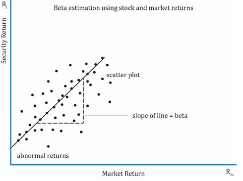
In a single-factor model, only one factor is considered. A classic single factor model is the market model which is given by this equation:

$R_i = \alpha_i + \beta R_m + e_i$

where: R_iis the dependent variable and R_m is the independent variable.

According to the market model, a stock’s return can be decomposed into:

α_i– Excess returns of the stock (difference between expected and realized returns).
β – Systematic risk of a security or the stock’s sensitivity to the market. For instance, how the stock’s return varies when the market return moves up or down by 1%.
R_m – Return on the market.
e_i– Error term that affects stock returns due to firm-specific factors. There is an error term because not all of a stock’s returns can be explained by market returns.

7. Calculation and Interpretation of Beta

Beta is a measure of systematic (or market) risk. Beta is a number and has no unit of measure. It tells us how sensitive an asset’s return is to the market as a whole. Beta determines the amount by which a stock’s return is expected to move for every 1 per cent increase or decrease in the market return. Beta is the ratio of the covariance of returns of stock i with returns on the market to the variance of market return.

β = $\frac{Cov(i,M)}{\sigma_M^2} = \frac{\rho_{iM} * \sigma_i}{\sigma_M}$

Interpretation of beta values:

β > 0: Return of the asset follows the market trend.
β < 0: Return of the asset moves in an opposite direction to the market trend (negatively correlated with the market).
β = 0: An asset’s return has no correlation with the market. For example, a risk-free asset has a beta of zero.
β = 1: Beta of market is equal to 1. If a stock has a beta of 1, it means it has the same volatility as that of the market.

How do we estimate beta:

Beta is estimated using a statistical method called linear regression analysis where stock returns are regressed against market returns. Historical security returns and historical market returns are used as inputs in this method. Let’s say, we consider a stock’s returns for the past 100 months. The pairs (security, market return) are plotted to get a scatter plot. Each point on the graph represents a month. A regression line is drawn though the scatter plot that best represents the data points. The point where the line intercepts the y-axis is α (or excess returns). The slope of the line is equal to its beta.

A portfolio beta is calculated as the weighted average beta of the individual securities in the portfolio.

Example

Assuming the standard deviation of market returns is 20%, calculate the beta for the following assets:

6-month T-bill.
A commodity with ? = 15%, and zero correlation with the market.
A stock with ? = 25% and correlation with the market = 0.6.

Solution:

6-month T-bill: beta for a T-bill is zero as there is no correlation between a risk-free asset and the market.
A commodity with ? = 15%, and zero correlation with the market: using equation 7, we can conclude that beta is zero if correlation with the market is zero.
A stock with ? = 25% and correlation with the market = 0.6: β = $\frac{0.6 * 0.25}{0.2}$ = 0.75

8. Capital Asset Pricing Model: Assumptions and the Security Market Line

The capital asset pricing model is a model used to calculate the expected rate of return of a risky asset, and gives the relationship between a security’s return and risk. CAPM states that the expected return of assets reflects only their systematic risk, which is measured by beta. Systematic or market risk cannot be diversified. It means that two assets with same beta will have the same expected return irrespective of their individual characteristics.

$r_e=R_f+\beta [E(R_{mkt}) - R_f]$

where:

$r_e$ = expected return

$R_f$ = risk-free rate

$\beta$ = systematic risk of security

$E ({R_{mkt})$ = expected return of market

$E ({R_{mkt}) - R_f$ = market risk premium; it is the compensation for assuming market risk.

8.1 Assumptions of the CAPM

We will now take a look at the assumptions for arriving at CAPM:

Investors are risk-averse, utility-maximizing, rational individuals.
Risk aversion means investors expect to be compensated for bearing risk. Different investors have different levels of risk aversion or risk tolerance. Utility maximizing means investors prefer higher returns to lower returns. Individuals are rational means that all investors have the ability to gather and process information to make logical decisions. In reality, however, this is not true for most investors as personal biases and experiences shroud their judgment.

Markets are frictionless. There are no transaction costs and no taxes.
Investors can borrow and lend as much as they want at the risk-free rate. One important assumption here is that there are no costs or restrictions on short-selling, which is not true in reality. This limits the CAPM.

All investors plan for the same, single holding period.
CAPM is based on a single period instead of multiple periods because it is easy to calculate.

Investors have homogenous expectations.
All investors analyze securities using the same probability distribution to arrive at identical valuations. This means all investors use the same estimates for expected returns, variance, and correlation between assets. Since the expected returns and standard deviation for all investors is the same, they will arrive at the same optimal risky portfolio, or the market portfolio in the CML.

Investments are infinitely divisible.
Investors can hold a fraction of any asset. It means that they may invest as much as or little in any asset.

Investors are price takers.
CAPM assumes that there are many small investors who cannot influence the security prices. They are price takers.

Example

FFC’s standard deviation of returns is 25% and its correlation with the market is 0.6. The standard deviation of returns for the market is 20%. The expected market return is 10% and the risk free rate is 3%. What is FFC’s expected return?

Solution:

β = $\frac{\rho_{iM} * \sigma_i}{\sigma_M} = \frac{0.6 * 0.25}{0.2}$ = 0.75

$r_e = R_f + \beta[E(R_{mkt}) - R_f] r_e = 0.03 + 0.75[0.1 - 0.03] = 0.0825 r_e = 8.25%$

8.2 The Security Market Line

The security market line (SML) is a graphical representation of the capital asset pricing model and applies to all securities, whether they are efficient or not. The graph has beta on the x-axis and expected return on the y-axis.

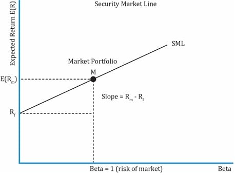
SML intersects y-axis at the risk-free rate.

Slope of the line = $\frac{R_m - R_f}{\beta} = R_m - R_f$

as β = 1 for the market. So, slope of the line is the market risk premium.

What is the difference between CML and SML?

Differences between CML and SML
CML	SML
Does not apply to all securities; applies to only efficient portfolios. Only systematic risk is priced. So CAL/CML can only be applied to those portfolios whose total risk is equal to systematic risk.	Applies to any security. It may include inefficient portfolios as well.
X-axis has the standard deviation of the portfolio.	X-axis has beta of the asset or portfolio.
R_p= R_f+ ( $\frac{R_m - R_f}{\sigma__m}$ ) * ?_p where ?_p is the total risk of the portfolio.	$r_e = R_f + \beta[E(R_{mkt}) - R_f]$ where β is the systematic risk. SML is just a graphical representation of CAPM.
Slope of the CML is the Sharpe ratio: $\frac{R_m - R_f}{\sigma__m}$	Slope of the SML is the market risk premium: $E(R_{mkt}) - R_f$
Similarities between CML and SML
Both CML and SML have expected portfolio return on the y-axis.
The line stretches from the risk-free asset to the market portfolio in both the cases.

Example

Ricky Ponting invests 10% in the risk-free asset, 40% in a mutual fund which tracks the market and 50% in a high-risk stock with a beta of 2.5. The risk-free rate is 5% and the expected market return is 10%. What is the portfolio beta and expected return?

Solution:

Risk- Free asset:	w = 0.1	r = 5%	β = 0
Mutual Fund:	w = 0.4	r = 10%	β = 1
High risk stock	w = 0.5	r = ?	β = 2.5

Portfolio beta = weighted average beta of all assets = 0.1 x 0 + 0.4 x 1 + 0.5 x 2.5 = 1.65

Portfolio return = $r_f + \beta (r_m - r_f)$

= 0.05 + 1.65 [0.1 – 0.05] = 0.1325 = 13.25%

Alternative method:

First determine the return of the high-risk stock using its beta.

Expected return of high-risk stock = 0.05 + 2.5[0.1 – 0.05] = 0.175 = 17.5%

Portfolio return= weighted average return of all assets = 0.1 x 5 + 0.4 x 10 + 0.5 x 17.5 = 13.25%

9. Capital Asset Pricing Model: Applications

The CAPM is important both from a theoretical and practical perspective. In this section, we will look at some of the practical applications of CAPM in capital budgeting, performance appraisal, and security selection.

Estimate of Expected Return

Given an asset’s systematic risk, the expected return can be calculated using CAPM.

To estimate the current price of an asset, we discount future cash flows at the required rate of return calculated using CAPM.
The required rate of return from the CAPM rate is also used in the capital budgeting process and to determine if a project is economically feasible.