
This reading covers:
Return can come in two forms:
We now look at the various types of return measures and their applicability.
Holding Period Return
Holding period return is the return earned on an asset during the period it was held. It is calculated as a sum of capital gain (price appreciation) and periodic income.
HPR = 
where:
PT – P0 = capital gain component
DT = dividend or income earned during period T
PT = price at end of period
P0 = price at beginning of period
Arithmetic or Mean Return
Arithmetic return is a simple arithmetic average of returns. Assume you have three stocks A, B, C with returns of 10%, 20% and 30% respectively. The collective return from the three stocks is (10 + 20 + 30)/3 = 20%.
Geometric Mean Return
Geometric mean return is the compounded rate of return earned on an investment.
Geometric mean return = [(1 + Ri1) * (1 + Ri2) * …….* (1 + RiT)] – 1
– 1
Assume you have a stock A which returns 10%, 20% and 30% in years 1, 2, and 3 respectively.
What is the mean return earned?
Geometric mean return = [(1.1) (1.2) (1.3)]0.333 – 1 = 19.7%
Money-weighted return is the internal rate of return on money invested that considers the cash inflows and cash outflows, and calculates the return on actual investment.
Money-weighted return is a useful performance measure when the investment manager is responsible for the timing of cash flows. This is often the case for private equity fund managers.
Example
Given the data below, compute the holding period return, arithmetic mean return, geometric mean return, and money-weighted return. Assume no withdrawals except at the end of year 3.
| Year | Assets under management at start of year (millions of $) | Net return |
| 1 | 30 | 10% |
| 2 | 33 | -5% |
| 3 | 35 | 15% |
Solution:
Holding period return:
Holding period = 3 years
Return = 1.1 x 0.95 x 1.15 = 1.20175 = 20.175%
Arithmetic mean:
Return = (10 – 5 + 15)/3 = 6.67%
Geometric mean:
Return = 
Money-weighted return:
To calculate the money-weighted return, we must know the net cash flows (cash inflows and outflows) for every year. So, let us draw a table and fill in the values and derive some others (in italics) to get the values for CF0, CF1, CF2, and CF3.
| Year 1 | Year 2 | Year 3 | |
| Balance from previous year | 0 | 33.00 | 31.35 |
| New investment by investor | 30.00 | 0 | 3.65 |
| Withdrawal by investor | 0 | 0 | 0 |
| Net balance at start of year | 30.00 | 33.00 | 35.00 |
| Investment return for year | 10% | -5% | 15% |
| Investment gain (loss) | 3.00 | (1.65) | 5.25 |
| Balance at end of year | 33.00 | 31.35 | 40.25 |
Now that we have the cash flows for the three years, let’s use the financial calculator to calculate IRR. CF0 = -30; CF1 = -3.84; CF2 = 0; CF3 = 40.25
IRR = 6.62%
The time-weighted rate of return measures the compound growth rate of $1 initially invested in the portfolio over a stated measurement period.
The time-weighted return can be calculated using the following steps:
Consider the following example:
| Time | Outflow | Inflow |
| 0 | $20.00 to purchase the first share | |
| 1 | $22.50 to purchase the second share | $0.50 dividend received on first share |
| $1.00 dividends ($0.50 x 2 shares);
$47.00 from selling 2 shares @ $23.50 per share |
Calculating the TWRR for this example is relatively simple because cash flows only occur at the start/end of every year. We will follow the steps mentioned earlier:
Steps 1: Break into evaluation period and value the portfolio at start/end of every period.
Step 2: Calculate the holding period return on the portfolio for each sub-period.
Step 3: Link or compound holding period returns to obtain an annual rate of return for the year.
Step 4: If the investment is for more than a year, take the geometric mean of the annual returns to obtain the time-weighted rate of return over that measurement period.
The TWRR is calculated as: = 0.1077 = 10.77%.
Money-weighted v/s time-weighted returns
Annualized return converts the returns for periods that are shorter or longer than a year, to an annualized number for easy comparison.
Annualized Return = (1 + rperiod)c – 1
Where
c = number of periods in year
Gross Return
Gross return is the return earned by an asset manager prior to deducting management fees and taxes. It measures the investment skill of a manager.
Net Return
Net return is the return earned by the investor on an investment after all managerial and administrative expenses have been accounted for. This is the measure of return that should matter to an investor.
Assume an investment manager generates $120 for every $100, and charges a 2% fee for management and administrative expenses. The gross return, in this case, is 20% and the net return is 18%.
Pre-tax and After-tax Nominal Return
The returns we saw till now were pre-tax nominal returns, i.e., before deducting any taxes or any adjustments for inflation. This is the default, unless otherwise stated.
After-tax nominal return is the return after accounting for taxes. The actual return an investor earns should consider the tax implications as well.
In the example that we saw above for gross and net return, 18% was the pre-tax nominal return. If the tax rate for the investor is 33.33%, then the after-tax nominal return will be 18(1 – 0.3333) = 12.0006%.
Real Return
Real return is the return after deducting taxes and inflation.
(1 + r) = (1 + rreal) (1 + π)
where:
rreal = real rate
π = rate of inflation
r = nominal rate
In the previous example, the after-tax nominal return was 12%. Assume the inflation rate for the period is 10%. What is the real rate of return?
Using the above formula, (1 + 0.12) = (1 + r) (1 + 0.1). Solving for r, we get 1.818%.
Instructor’s tip: If the answer choices are close to each other, use this formula to determine the correct answer. Else, you may use an approximation to solve for r quickly as nominal rate = real rate + inflation.
Leveraged Return
In cases, where an investor borrows money to invest in assets like bonds or real estate, the leveraged return is the return earned by the investor on his money after accounting for interest paid on borrowed money.
Portfolio Expected Return and Variance
For a two-asset portfolio, the expected return and variance can be computed as:
E(RP) = w1R1 + w2R2
𝜎p2 = w12 𝜎12 + w22 𝜎22 + 2 w1 w2 𝜎1 𝜎2 ρ
Example
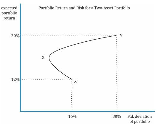
My portfolio consists of two stocks X and Y. X represents 60% of the portfolio and Y the remaining 40%. X has an expected return of 12% and a standard deviation of 16%. Y has an expected return of 20% and a standard deviation of 30%. The correlation is 0.5. What is the expected return and risk of my portfolio? How does the return/risk change when the weights of X and Y change?
Solution:
E(RP) = w1 R1 + w2 R2
E(RP )= 0.6 x 12 + 0.4 x 20 = 15.2%
We can calculate the portfolio variance:
𝜎p2 = (0.6)2 (0.16)2 + (0.4)2 (0.3)2 + 2 (0.6) (0.4) (0.16) (0.3) (0.5) = 0.0351
𝜎p = 0.1874 = 18.74%
To understand how return/risk change when the weights of X and Y change, we will calculate the risk and return for different weights and plot a curve as shown in the graph below.
The graph below plots portfolio risk and return for a two-asset portfolio and shows the impact of correlation of assets on portfolio risk. As you can see, there is no risk-return trade-off when 100% is invested either in X or Y.


Ace the Exam with IFT Notes!

Ace the Exam with Active Learning!

Accelerate your studies!

Practice your way to success!
 Do IFT Mocks to make you exam-ready!


Sign up to get more!