
In this section, we look at two measures of interest rate risk: duration and convexity.
The duration of a bond measures the sensitivity of the bond’s full price (including accrued interest) to changes in interest rates. In other words, duration indicates the percentage change in the price of a bond for a 1% change in interest rates. The higher the duration, the more sensitive the bond is to change in interest rates. Duration is expressed in years.
There are two categories of duration: yield duration and curve duration.
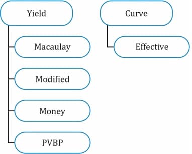
As indicated in the diagram above, there are several types of yield duration.
Macaulay duration is a weighted average of the time to receipt of the bond’s promised payments, where the weights are the shares of the full price that correspond to each of the bond’s promised future payments. Let us consider a 10-year, 8% annual payment bond. To determine the Macaulay duration, we calculate the present value of each cash flow, multiply by weight and add, as shown in the below exhibit
| Exhibit 2: Macaulay Duration of a 10 – Year, 8% Annual Payment Bond | ||||
| Period | Cash flow | Present Value | Weight | Period x Weight |
| 1 | 8 | 7.246377 | 0.08475 | 0.0847 |
| 2 | 8 | 6.563747 | 0.07677 | 0.1535 |
| 3 | 8 | 5.945423 | 0.06953 | 0.2086 |
| 4 | 8 | 5.385347 | 0.06298 | 0.2519 |
| 5 | 8 | 4.878032 | 0.05705 | 0.2853 |
| 6 | 8 | 4.418507 | 0.05168 | 0.3101 |
| 7 | 8 | 4.002271 | 0.04681 | 0.3277 |
| 8 | 8 | 3.625245 | 0.04240 | 0.3392 |
| 9 | 8 | 3.283737 | 0.03840 | 0.3456 |
| 10 | 108 | 40.154389 | 0.46963 | 4.6963 |
| 85.503075 | 1.00000 | 7.0029 | ||
We can also use the following formula to calculate Macaulay Duration:
![(\frac{1+r}{r} - \frac{1+r+[N*(c-r)]}{c*[(1+r)^N-1]+r}) - \frac{t}{T}](https://ift.world/wp-content/ql-cache/quicklatex.com-60056cd63e890aa0c3d221c3521d390f_l3.png "Rendered by QuickLaTeX.com")
where:
r = yield-to-maturity
t = number of days from the last coupon payment date to the settlement date
T = number of days in the coupon period
c = coupon rate per period
N = number of periods to maturity
Instructor’s Note:
Understanding how the Macaulay duration works is more important than memorizing the formula.
Modified duration provides an estimate of the percentage price change for a bond given a change in its yield-to-maturity. It represents a simple adjustment to Macaulay duration as shown in the equation below:

where: r is the yield per period.
Therefore, percentage price change for a bond given a change in its YTM can be calculated as:

The AnnModDur term is the annual modified duration, and the ΔYield term is the change in the annual yield-to-maturity. The ≈ sign indicates that this calculation is estimation. The minus sign indicates that bond prices and yields-to-maturity move inversely.
Example 8: Calculating the modified duration of a bond
A 2-year, annual payment, $100 bond has a Macaulay duration of 1.87 years. The YTM is 5%. Calculate the modified duration of the bond.
Solution:
Modified duration =1.87/(1 + 0.05) = 1.78 years
The percentage change in the price of the bond for a 1% increase in YTM will be:
-1.78 * 0.01 * 100 = -1.78%.
Modified duration is calculated if the Macaulay duration is known. But there is another way of calculating an approximate value of modified duration: estimate the slope of the line tangent to the price-yield curve. This can be done by using the equation below:

where:
PV_ = price of the bond when yield is decreased;
PV0 = initial price of the bond
PV+ = price of the bond when yield is increased
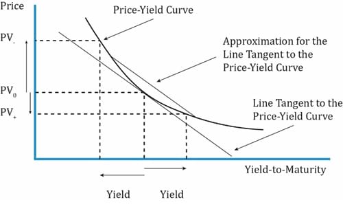
Interpretation of the diagram:
 denotes the original price of the bond.
 denotes the price of the bond when YTM is increased and PV_ denotes the bond price when YTM is decreased.
 and horizontal distance = 2 x Δ yield.
How to calculate approximate modified duration (or estimate the slope of the price-yield curve):
Once the approximate modified duration is known, the approximate Macaulay duration can be calculated using the formula below:
Approximate Macaulay Duration = Approximate Modified Duration x (1 + r)
Example 9: Calculating the approximate modified duration and approximate Macaulay duration
Assume that the 6% U.S. Treasury bond matures on 15 August, 2017 is priced to yield 10% for settlement on 15 November, 2014. Coupons are paid semiannually on 15 February and 15 August. The yield-to-maturity is stated on a street-convention semiannual bond basis. This settlement date is 92 days into a 184-day coupon period, using the actual/actual day-count convention. Compute the approximate modified duration and the approximate Macaulay duration for this Treasury bond assuming a 50bps change in the yield-to-maturity.
Solution:
The yield-to-maturity per semiannual period is 5% (=10/2). The coupon payment per period is 3% (= 6/2). When the bond is purchased, there are 3 years (6 semiannual periods) to maturity. The fraction of the period that has passed is 0.5 (=92/184).
The full price (including accrued interest) at a YTM of 5% is 92.07 per 100 of par value.
![PV_0 = [\frac{3}{(1.05)^1} + \frac{3}{(1.05)^2} +\frac{3}{(1.05)^3} +\frac{3}{(1.05)^4} +\frac{3}{(1.05)^5} +\frac{103}{(1.05)^6}] * (105)^{\frac{92}{184}}](https://ift.world/wp-content/ql-cache/quicklatex.com-e11279f2908dccfbfac9e8753bacb1a6_l3.png "Rendered by QuickLaTeX.com")

Increase the yield to maturity from 10% to 10.5% – therefore, from 5% to 5.25% per semiannual period, and the price becomes 90.97 per 100 of par value.
![\left PV_+ = [\frac{3}{(1.0525)^1} + \frac{3}{(1.0525)^2} + \frac{3}{(1.0525)^3} + \frac{3}{(1.0525)^4} + \frac{3}{(1.0525)^5} + \frac{103}{(1.0525)^6}] * (1.0525)^{\frac{92}{184}}](https://ift.world/wp-content/ql-cache/quicklatex.com-c982f5effb901cbfc48629478557cf63_l3.png "Rendered by QuickLaTeX.com")

Decrease the yield to maturity from 10% to 9.5% – therefore, from 5% to 4.75% per semiannual period, and the price becomes 93.19 per 100 of par value.
![PV_ = [\frac{3}{(1.0475)^1} + \frac{3}{(1.0475)^2} + \frac{3}{(1.0475)^3} + \frac{3}{(1.0475)^4} + \frac{3}{(1.0475)^5} + \frac{103}{(1.0475)^6}] * (1.0475)^{\frac{92}{184}}](https://ift.world/wp-content/ql-cache/quicklatex.com-9840b7f7d0ce5c8bc4c4fcc9b4d5fd46_l3.png "Rendered by QuickLaTeX.com")

The approximate annualized modified duration for the Treasury bond is 2.41
ApproxModDur = 
The approximate annualized Macaulay Duration is 2.53
ApproxModDur = 2.41 * 1.05 = 2.53
Therefore, from these statistics, the investor knows that the weighted average time to receipt of interest and principal payments is 2.53 years (the Macaulay Duration) and that the estimated loss in the bond’s market value is 2.41% (the Modified Duration) if the market discount rate were to suddenly go up by 1.0%.
Bonds with embedded options and mortgage backed securities do not have a well-defined YTM. These securities may be prepaid well before the maturity date. Hence, yield duration statistics are not suitable for these instruments. For such instruments, the best measure of interest rate sensitivity is the effective duration which measures the sensitivity of the bond’s price to a change in a benchmark yield curve (instead of its own YTM).

Difference between approx. modified duration and effective duration:
The denominator for approx. modified duration has the bond’s own yield-to-maturity. It measures the bond’s price change to changes in its own YTM. But, the denominator for effective duration has the change in the benchmark yield curve. It measures the interest rate risk in terms of change in benchmark yield curve.
Example 10: Calculating the effective duration
A Pakistani defined-benefit pension scheme seeks to measure the sensitivity of its retirement obligations to market interest rate changes. The pension scheme manager hires an actuarial consultant to model the present value of its liabilities under three interest rate scenarios
The following chart shows the results of the analysis:
| Interest Rate Assumption | Present Value of Liabilities |
| 9.5% | PKR 10.5 million |
| 10%
10.5% |
PKR 10 million
PKR 9 million |
Compute the effective duration of pension liabilities. PV0 = 10, PV+ = 9, PV– = 10.5, and Δ curve = 0.005. The effective duration of the pension liabilities is 15.
 = 15
= 15
This effective duration statistic for the pension scheme’s liabilities might be used in asset allocation decisions to decide the mix of equity, fixed income, and alternative assets.
Key rate duration is a measure of a bond’s sensitivity to a change in the benchmark yield curve at a specific maturity. This topic is covered in detail at Level II.
The duration measures we have seen so for assume a parallel shift in the yield curve. But what if the shift in the yield curve is not parallel? Here it is appropriate to use ‘Key rate duration’.
Key rate durations are used to identify “shaping risk” of a bond, which is a bond’s sensitivity to changes in the shape of the benchmark yield curve. For instance, analysts can analyze the interest rate sensitivity if the yield curve flattens or if the yield curve steepens.


Ace the Exam with Active Learning!

Ace the Exam with IFT Notes!
 Do IFT Mocks to make you exam-ready!

Accelerate your studies!

Practice your way to success!


Sign up to get more!