IFT Notes for Level I CFA^® Program

LM07 Introduction to Linear Regression

Part 1

1. Simple Linear Regression

Financial analysts often need to find whether one variable X can be used to explain another variable Y. Linear regression allows us to examine this relationship.

Suppose an analyst is evaluating the return on assets (ROA) for an industry. He gathers data for six companies in that industry.

Company	ROA (%)
A	6
B	4
C	15
D	20
E	10
F	20

Range = 4% to 20%

Average value = 12.5%

Let Y represents the variable we are trying to explain (in this case ROA), Y_i represents a particular observation, and $\underline{Y}$ represent the mean value. Then the variation of Y can be expressed as:

Variation of Y= $\sum^N_{i=1}{}{\ \left(Y_i-\ \underline{Y}\right)}^{\ 2}$

The variation of Y is also called sum of squares total (SST) or the total sum of squares. Our aim is to understand what explains the variation of Y.

The analyst now wants to check if another variable – CAPEX can be used to explain the variation of ROA. The analyst defines CAPEX as: capital expenditures in the previous period, scaled by the prior period’s beginning property, plant, and equipment. He gathers the following data for the six companies:

Company	ROA (%)	CAPEX(%)
A	6	0.7
B	4	0.4
C	15	5.0
D	20	10.0
E	10	8.0
F	20	12.5
Arithmetic mean	12.50	6.10

The relation between the two variables can be visualized using a scatter plot.

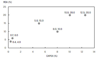
The variable whose variation we want to explain, also called the dependent variable is presented on the vertical axis. It is typically denoted by Y. In our example ROA is the dependent variable.

The explanatory variable, also called the independent variable is presented on the horizontal axis. It is typically denoted by X. In our example CAPEX is the independent variable.

A linear regression model computes the best fit line through the scatter plot, which is the line with the smallest distance between itself and each point on the scatter plot. The regression line may pass through some points, but not through all of them.

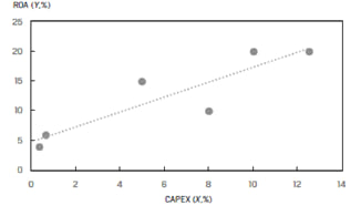
Regression analysis with only one independent variable is called simple linear regression (SLR). Regression analysis with more than one independent variable is called multiple regression. In this reading we focus on single independent variable, i.e., simple linear regression.

2. Estimating the Parameters of a Simple Linear Regression

2.1 The Basics of Simple Linear Regression

Linear regression assumes a linear relationship between the dependent variable (Y) and independent variable (X). The regression equation is expressed as follows:

$Y_i=b_0+b_1X_i+{\varepsilon }_i$

where:

i = 1, …, n

Y = dependent variable

b₀ = intercept

b₁ = slope coefficient

X = independent variable

ε = error term

b₀ and b₁ are called the regression coefficients.

The equation shows how much Y changes when X changes by one unit.

2.2 Estimating the Regression Line

Linear regression chooses the estimated values for intercept and slopesuch that the sum of the squared errors (SSE), i.e., the vertical distances between the observations and the regression line is minimized.

This is represented by the following equation. The error terms are squared so that they don’t cancel out each other. The objective of the model is that the sum of the squared error terms should be minimized.

SSE= $\sum^N_{i=1}{}\ {\left(Y_i-\ {\hat{Y}}_i\right)}^2=\sum^N_{i=1}{}\ {\left[Y_i-({\hat{b}}_0+\ {\hat{b}}_1X_i)\right]}^2$

The slope coefficient is calculated as:

${\hat{b}}_1=\frac{Covairance\ of\ Yand\ X}{Variance\ of\ X}$

= $\frac{\frac{\sum^N_{i=1}{}\left(Y_i-\ \underline{Y}\right)\left(X_i-\ \underline{X}\right)\ }{n-1}}{\frac{\sum^N_{i=1}{}\ {\left(X_i-\ \underline{X}\right)}^2}{n-1}}$

= $\frac{\sum^N_{i=1}{}\left(Y_i-\ \underline{Y}\right)\left(X_i-\ \underline{X}\right)\ }{\sum^N_{i=1}{}\ {\left(X_i-\ \underline{X}\right)}^2}$

Note: This formula is similar to correlation which is calculated as:

$r=\frac{Covairance\ of\ Yand\ X}{(Std\ dev\ of\ X)(Std\ dev\ of\ Y)}$

Once we calculate the slope, the intercept can be calculated as:

Note: On the exam you will most likely be given the values of b₁ and b₀. It is unlikely that you will be asked to calculate these values. Nevertheless, the following table shows how to calculate the slope and intercept.

Company	ROA(Y_i)	CAPEX (X_i)
A	6.0	0.7	42.25	29.16	35.10
B	4.0	0.4	72.25	32.49	48.45
C	15.0	5.0	6.25	1.21	-2.75
D	20.0	10.0	56.25	15.21	29.25
E	10.0	8.0	6.25	3.61	-4.75
F	20.0	12.5	56.25	40.96	48.00
Sum	75.0	36.6	239.50	122.64	153.30
Mean	12.5	6.100

Slope coefficient: ${\hat{b}}_1=\frac{153.30}{122.64}$ = 1.25

Intercept: ${\hat{b}}_0=12.5-\left(1.25\ x\ 6.10\right)$ = 4.875

The regression model can thus be expressed as:

$Y_i=4.875+1.25X_i+{\varepsilon }_i$

2.3 Interpreting the Regression Coefficients

The intercept is the value of the dependent variable when the independent variable is zero. In our example, if a company makes no capital expenditures, its expected ROA is 4.875%.

The slope measures the change in the dependent variable for a one-unit change in the independent variable. If the slope is positive, the two variables move in the same direction. If the slope is negative, the two variables move in opposite directions. In our example, if CAPEX increases by one unit, ROA increases by 1.25%.

2.4 Cross-Sectional vs. Time-Series Regressions

Regression analysis can be used for two types of data:

Cross sectional data: Many observations for different companies, asset classes, investment funds etc. for the same time period.
Time-series data: Many observations from different time periods for the same company, asset class, investment funds etc.

3. Assumptions of the Simple Linear Regression Model

The simple linear regression model is based on the following four assumptions:

Linearity: The relationship between the dependent variable, Y, and the independent variable, X, is linear.
Homoskedasticity: The variance of the regression residuals is the same for all observations.
Independence: The observations, pairs of Ys and Xs, are independent of one another. This implies the regression residuals are uncorrelated across observations.
Normality: The regression residuals are normally distributed.

3.1 Assumption 1: Linearity

Since we are fitting a straight line through a scatter plot, we are implicitly assuming that the true underlying relationship between the two variables is linear.

If the relationship between the variables is non-linear, then using a simple linear regression model will produce invalid results.

Exhibit 10 from the curriculum shows two variables that have an exponential relationship. A linear regression line does not fit this relationship well. At lower and higher values of X, the model underestimates Y. Whereas, at middle values of X, the model overestimates Y.

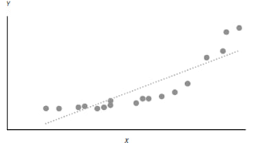
Another point related to this assumption is that the independent variable X should not be random. If X is random, there would be no linear relationship between the two variables.

Also, the residuals of the model should be random. They should not exhibit a pattern when plotted against the independent variable. As shown in Exhibit 11, the residuals from the linear regression model in Exhibit 10 do not appear random.

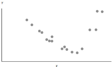
Hence, a linear regression model should not be used for these two variables.

3.2 Assumption 2: Homoskedasticity

Assumption#2 is that the variance of the residuals is constant for all observations. This condition is called homoskedasticity. If the variance of the error term is not constant, then it is called heteroskedasticity.

Exhibit 12 shows a scatter plot of short-term interest rates versus inflation rate for a country. The data represents a total span of 16 years. We will refer to the first eight years of normal rates as Regime 1 and the second eight years of artificially low rates as Regime 2.

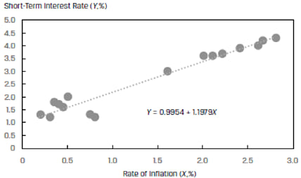
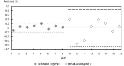
At first glance, the model seems to fit the data well. However, when we plot the residuals of the model against the years, we can see that the residuals for the two regimes appear different. This is shown in Exhibit 13 below. The variation in residuals for Regime 1 is much smaller than the variation in residuals for Regime 2. This is a clear violation of the homoskedasticity assumption and the two regimes should not be clubbed together in a single model.

3.3 Assumption 3: Independence

Assumption# 3 states that the residuals should be uncorrelated across observations. If the residuals exhibit a pattern, then this assumption will be violated.

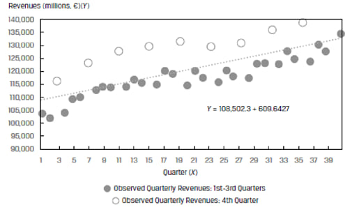
For example, Exhibit 15 from the curriculum plots the quarterly revenues of a company over 40 quarters. The data displays a clear seasonal pattern. Quarter 4 revenues are considerably higher than the first 3 quarters.

A plot of the residuals from this model in Exhibit 16 also helps us see this pattern. The residuals are correlated – they are high in Quarter 4 and then fall back in the other quarters.

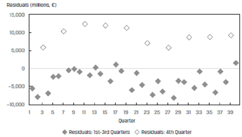
Both exhibits show that the assumption of residual independence is violated and the model should not be used for this data.

3.4 Assumption 4: Normality

Assumption#4 states that the residuals should be normally distributed.

Instructor’s Note: This assumption does not mean that X and Y should be normally distributed, it only means that the residuals from the model should be normally distributed.

4. Analysis of Variance

4.1 Breaking down the Sum of Squares Total into Its Components

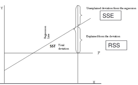
To evaluate how well a linear regression model explains the variation of Y we can break down the total variation in Y (SST) into two components: Sum of square errors (SSE) and regression sum of squares (RSS).

Total sum of squares (SST) $\sum^N_{i=1}{}{\ \left(Y_i-\ \underline{Y}\right)}^{\ 2}$ : , : This measures the total variation in the dependent variable. SST is equal to the sum of squared distances between the actual values of Y and the average value of Y.

The regression sum of squares (RSS) ${\sum^N_{i\ =\ 1}{}\ (\widehat{Y_i}-\underline{Y})}^2$ . , . This is the amount of total variation in Y that is explained in the regression equation. RSS is the sum of squared distances between the predicted values of Y and the average value of Y.

The sum of squared errors or residuals (SSE) $\ \sum^{N\ \ }_{i\ =\ 1}{}{\ \left(Y_i-\widehat{Y_i}\right)}^2$ .,.This is also known as residual sum of squares. It measures the unexplained variation in the dependent variable. SSE is the sum of the vertical distances between the actual values of Y and the predicted values of Y on the regression line.

SST = RSS + SSE

i.e., Total variation = explained variation + unexplained variation

These concepts are illustrated in the figure below:

4.2 Measures of Goodness of Fit

Goodness of fit indicates how well the regression model fits the data. Several measures are used to evaluate the goodness of fit.

Coefficient of determination: The coefficient of determination, denoted by R², measures the fraction of the total variation in the dependent variable that is explained by the independent variable.

$R^2=\frac{Explained\ variation}{Total\ variation}=\frac{Regression\ sum\ of\ squares\ (RSS)}{Sum\ of\ squares\ total\ (SST)}$

Characteristics of coefficient of determination, :

The higher the R², the more useful the model. R² has a value between 0 and 1. For example, if R² is 0.03, then this explains only 3% of the variation in the independent variable and the explanatory power of the model is low. However, if R² is 0.85, the model explains over 85% of the variation and the explanatory power of the model is high.

It tells us how much better the prediction is by using the regression equation rather than just $\underline{y}$ (average value) to predict y.

With only one independent variable, is the square of the correlation between X and Y.

The correlation, r, is also called the “multiple-R”.

F-test: For a meaningful regression model, the slope coefficients should be non-zero. This is determined through the F-test which is based on the F-statistic. The F-statistic tests whether all the slope coefficients in a linear regression are equal to 0. In a regression with one independent variable, this is a test of the null hypothesis H_0: b₁ = 0 against the alternative hypothesis H_a: b₁≠ 0.

The F-statistic also measures how well the regression equation explains the variation in the dependent variable. The four values required to construct the F-statistic for null hypothesis testing are:

The total number of observations (n)
The total number of independent variables (k)
The regression sum of squares (RSS)
The sum of squared errors or residuals (SSE)

The F-statistic is calculated as:

F = $\frac{\frac{RSS}{k}}{\frac{SSE}{n-(k+1)}}$ = $\frac{Mean\ square\ regression}{Mean\ square\ error}$ = $\frac{MSR}{MSE}$

Interpretation of F-test statistic:

The higher the F-statistic, the better.
A high F-statistic implies that the regression model does a good job of explaining the variation in the dependent variable.
A low F-statistic implies that the regression model does not do a good job of explaining the variation in the dependent variable.
An F-statistic of 0 indicates that the independent variable does not explain variation in the dependent variable.

4.3 ANOVA and Standard Error of Estimate in Simple Linear Regression

Analysis of variance or ANOVA is a statistical procedure of dividing the total variability of a variable into components that can be attributed to different sources. We use ANOVA to determine the usefulness of the independent variable or variables in explaining variation in the dependent variable.

ANOVA table

Source of variation	Degrees of freedom	Sum of squares	Mean sum of squares	F-statistic
Regression (explained variation)	k	RSS	MSR = (RSS/k)	F = (MSR/MSE)
Error (unexplained variation)	n – 2	SSE	MSE = [SSE/(n-k-1)]
Total variation	n – 1	SST

n represents the number of observations and k represents the number of independent variables. With one independent variable, k = 1. Hence, MSR = RSS and MSE = SSE / (n – 2).

Information from the ANOVA table can be used to compute the standard error of estimate (SEE). The standard error of estimate (SEE) measures how well a given linear regression model captures the relationship between the dependent and independent variables. It is the standard deviation of the prediction errors. A low SEE implies an accurate forecast.

The formula for the standard error of estimate is given below:

Standard error of estimate (SEE)= √MSE

A low SEE implies that the error (or residual) terms are small and hence the linear regression model does a good job of capturing the relationship between dependent and independent variables.

The following example demonstrates how to interpret an ANOVA table.

Example: Using ANOVA Table Results to Evaluate a Simple Linear Regression

(This is based on Example 5 from the curriculum.)

You are provided the following ANOVA table:

Source	Sum of Squares	Degrees of Freedom	Mean Square
Regression	576.1485	1	576.1485
Error	1,873.5615	98	19.1180
Total	2,449.7100

What is the coefficient of determination for this regression model?
What is the standard error of the estimate for this regression model?
At a 5% level of significance, do we reject the null hypothesis of the slope coefficient equal to zero if the critical F-value is 3.938?
Based on your answers to the preceding questions, evaluate this simple linear regression model.

Solution to 1: Coefficient of determination (R²) = RSS / SST = 576.148/2,449.71 = 23.52%.

Solution to 2: Standard error of estimate (SEE)= √MSE= √19.1180=4.3724

Solution to 3:

F = (MSR/MSE) = (576.1485/19.1180) = 30.1364

Since the calculated F-stat is higher than the critical value of 3.938, we can conclude that the slope coefficient is statistically different from 0.

Solution to 4: The coefficient of determination indicates that the model explains 23.52% of the variation in Y. Also, the F-stat confirms that the model’s slope coefficient is statistically different from 0. Overall, the model seems to fit the data reasonably well.