LM04 Common Probability Distributions

Part 2

4.  Normal Distribution

The normal distribution is the most extensively used probability distribution in quantitative work. A normal distribution is symmetrical and bell-shaped as shown in the graph below:

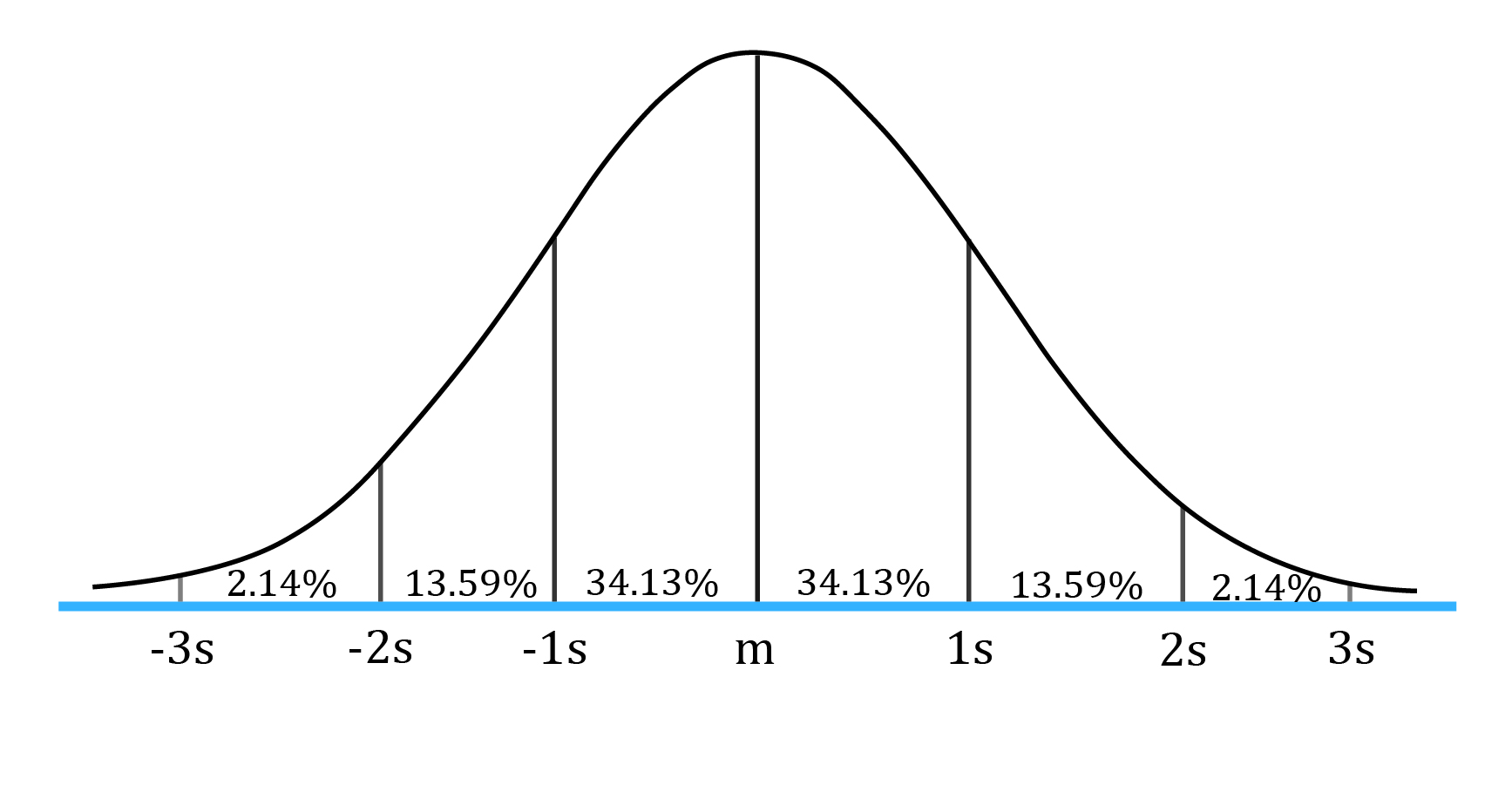
In this figure ‘m’ stands for mean, 1s means one standard deviation, 2s means two standard deviations, and so on. We can make the following probability statements for a normal distribution:

• Approximately 68% of all observations fall in the interval m ± 1s.
• Approximately 95% of all observations fall in the interval m ± 2s.
• Approximately 99% of all observations fall in the interval m ± 3s.

The intervals indicated above are easy to remember but are only approximate for the stated probabilities. More precise intervals (confidence intervals) are:

• 90% of all observations are in the interval m ± 1.65s.
• 95% of all observations are in the interval m ± 1.96s.
• 99% of all observations are in the interval m ± 2.58s.

The characteristics of a normal distribution are as follows:

• The normal distribution is completely described by two parameters – its mean, µ, and variance, σ². We indicate this as X ~ N (µ, σ ²).
• The normal distribution has a skewness of 0 (it is symmetric) and a kurtosis (measure of peakedness) of 3. Due to the symmetry, the mean, median and mode are all equal for a normal random variable.
• A linear combination of two or more normal random variables is also normally distributed.

Standard normal distribution

The normal distribution with mean (µ) = 0 and standard deviation (σ) = 1 is called the standard normal distribution.

The formula for standardizing a random variable X is:

where:

µ is the population mean.

σ is the population standard deviation.

The Z-table is used to find the probability that X will be less than or equal to a given value. Suppose we have a normal random variable, X, with µ = 10 and σ = 2. If the value of X is 11, we standardize X with Z = (11 – 10)/2 = 0.5.

The probability that we will observe a value less than 11 for X ~ N (10, 2) is exactly the same as the probability that we will observe a value less than 0.5 for Z ~ N (0, 1).

We can answer probability questions about X using standardized values and probability tables for Z. A snapshot of a table showing cumulative probabilities for a standard normal distribution is shown below.

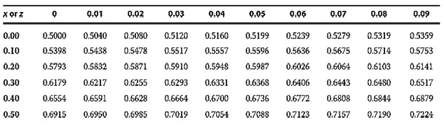
To find the probability that a standard normal variable is less than or equal to 0.5, for example, locate the row that contains 0.50, look at the 0 column, and find the entry 0.6915. Thus, P(Z ≤ 0.5) = 0.6915 or 69.15%.

The probability that a standard normal variable is less than or equal to 0 is 0.5000.  This is true by definition because the mean of a standard normal distribution is 0.  The table above validates this fact.

For a non-negative number x, we can use N(x) directly from the table. For a negative number –x, N(-x) = 1.0 – N(x).  Essentially, we are using the fact that the normal distribution is symmetric around the mean.

Example

A portfolio has a mean return of 15% and a standard deviation of return of 20% per year. What is the probability that the portfolio return would be below 18%? We are given the following information from the z-table: P(Z < 0.15) = 0.5596, P(Z > 0.15) = 0.4404, P(Z < 0.18) = 0.5714, P(Z > 0.18) = 0.4286.

Solution:

Univariate v/s multivariate distribution

Univariate distribution

A univariate distribution describes the probability distribution of a single random variable. For example, the distribution of expected return of one stock from a portfolio.

Multivariate distribution

A multivariate distribution describes the probability distribution for a group of related random variables. For example, the distribution of expected return of a portfolio with multiple stocks.

A multivariate normal distribution for the returns on n stocks is completely defined by the following three sets of parameters:

• Mean returns on the individual stocks (n means in total).
• Variances of the individual stocks (n variances in total).
• Pairwise return correlations between the stocks (n (n – 1)/2 distinct correlations in total).

Share on :