IFT Notes for Level I CFA^® Program

LM06 Hypothesis Testing

Part 3

9. Tests Concerning a Single Mean

One of the decisions we need to make in hypothesis testing is deciding which test statistic and which corresponding probability distribution to use. We use the following table to make this decision:

Sampling from		Small sample size (n<30)	Large sample size (n≥30)
Normal distribution	Variance known	z	z
Normal distribution	Variance unknown	t	t (or z)
Non –normal distribution	Variance known	NA	z
Non –normal distribution	Variance unknown	NA	t (or z)

If the population variance is known and our sample size is large, we can use the z-statistic and z-distribution to compute the critical value.

However, if we do not know the population variance and we have a small sample size, then we have to use the t-statistic and t-distribution to compute the critical values.

Example

An analyst believes that the average return on all Asian stocks was less than 2%. The sample size is 36 observations with a sample mean of -3. The standard deviation of the population is 4. Will he reject the null hypothesis at the 5% level of significance?

Solution:

In this case, our null and alternative hypotheses are:

H₀: µ ≥ 2

H_a: µ < 2

The standard error of the sample is: ${\sigma }_{\overline{x}\ }$ = $\frac{\sigma }{\sqrt{n}}$ = $\frac{4}{\sqrt{36}}$ = 0.67

The test statistic is:

test statistic = $\frac{sample\ statistic-value\ of\ the\ parameter\ under\ H_0}{standard\ error\ of\ the\ sample\ statistic}$ = $\frac{-3-2}{0.67}$ = -7.5

The critical values corresponding to a 5% level of significance is -1.65.

When we consider the left tail of the distribution, our decision rule is as follows: Reject the null hypothesis if the test statistic is less than the critical value and vice versa. Since our calculated test statistic of -7.5 is less than the critical value of -1.65, we reject the null hypothesis.

Example

Fund Alpha has been in existence for 20 months and has achieved a mean monthly return of 2% with a sample standard deviation of 5%. The expected monthly return for a fund of this nature is 1.60%. Assuming monthly returns are normally distributed, are the actual results consistent with an underlying population mean monthly return of 1.60%?

Solution:

The null and alternative hypotheses for this example will be:

H₀: µ = 1.60 versus H_a: µ ≠ 1.60

test statistic = $\frac{\overline{X}-{\mu }_0}{\frac{s}{\sqrt{n}}}$ = $\frac{2-1.60}{\frac{5}{\sqrt{20}}}$ = 0.36

Using this formula, we see that the value of the test statistic is 0.36.

The critical values at a 0.05 level of significance can be calculated from the t-distribution table. Since this is a two-tailed test, we should look at a 0.05/2 = 0.025 level of significance with df = n – 1 = 20 – 1 = 19. This gives us two values of -2.1 and +2.1.

Since our test statistic of 0.35 lies between -2.1 and +2.1, i.e., the acceptance region, we do not reject the null hypothesis.

10. Test Concerning Differences Between Means with Independent Samples

Instructor’s Note:

Focus on the basics of this topic, the probability of being tested on the details is low.

In this section, we will learn how to calculate the difference between the means of two independent and normally distributed populations. We perform this test by drawing a sample from each group. If it is reasonable to believe that the samples are normally distributed and also independent of each other, we can proceed with the test. We may also assume that the population variances are equal or unequal. However, the curriculum focuses on tests under the assumption that the population variances are equal.

The test statistic is calculated as:

t = $\frac{\left({\overline{X}}_1-\ {\overline{X}}_2\right)-({\mu }_1-{\mu }_2)}{(\frac{s^2_p}{n_1}+\ \frac{s^2_p}{n_2})^{1/2}}$

The term s_p² is known as the pooled estimator of the common variance. It is calculated by the following formula:

$s^2_p$ = $\frac{\left(n_1-\ 1\right)s^2_1+\left(n_2-\ 1\right)s^2_2}{n_1{+\ n}_2-2}$

The number of degrees of freedom is n₁ + n₂ – 2.

Example

(This is based on Example 9 from the curriculum.)

An analyst wants to test if the returns for an index are different for two different time periods. He gathers the following data:

		Period 1	Period 2
Mean		0.01775%	0.01134%
Standard deviation		0.31580%	0.38760%
	Sample size	445 days	859 days

Note that these periods are of different lengths and the samples are independent; that is, there is no pairing of the days for the two periods.

Test whether there is a difference between the mean daily returns in Period 1 and in Period 2 using a 5% level of significance.

Solution:

The first step is to formulate the null and alternative hypotheses. Since we want to test whether the two means were equal or different, we define the hypotheses as:

H₀: µ₁ – µ₂ = 0

H_a: µ₁ – µ₂ ≠ 0

We then calculate the test statistic:

$s^2_p$ = $\frac{\left(n_1-\ 1\right)s^2_1+\left(n_2-\ 1\right)s^2_2}{n_1{+\ n}_2-2}$ = $\frac{\left(445-1\right)09973+\left(859-1\right)15023}{445+859-2}$ = 0.1330

t= $\frac{\left({\overline{X}}_1-\ {\overline{X}}_2\right)-({\mu }_1-{\mu }_2)}{(\frac{s^2_p}{n_1}+\ \frac{s^2_p}{n_2})^{1/2}}$ = $\frac{\left(0.01775-0.01134\right)-0}{(\frac{0.1330}{445}+\ \frac{0.1330}{859})^{1/2}}$ =0.3099

For a 0.05 level of significance, we find the t-value for 0.05/2 = 0.025 using df = 445 + 859 – 2=1302. The critical t-values are ±1.962. Since our test statistic of 0.3099 lies in the acceptance region, we fail to reject the null hypothesis.

We conclude that there is insufficient evidence to indicate that the returns are different for the two time periods.

11. Test Concerning Differences Between Means with Dependent Samples

Instructor’s Note:

Focus on the basics of this topic, the probability of being tested on the details is low.

In the previous section, in order to perform hypothesis tests on differences between means of two populations, we assumed that the samples were independent. What if the samples are not independent? For example, suppose you want to conduct tests on the mean monthly return on Toyota stock and mean monthly return on Honda stock. These two samples are believed to be dependent, as they are impacted by the same economic factors.

In such situations, we conduct a t-test that is based on data arranged in paired observations. Paired observations are observations that are dependent because they have something in common.

We will now discuss the process for conducting such a t-test.

Example:

Suppose that we gather data regarding the mean monthly returns on stocks of Toyota and Honda for the last 20 months, as shown in the table below:

Month	Mean return of Toyota stock	Mean monthly return of Honda stock	Difference in mean monthly returns (d_i)
1	0.5%	0.4%	0.1%
2	0.7%	1.0%	-0.3%
3	0.3%	0.7%	-0.4%
…	…	…	…
20	0.9%	0.6%	0.3%
Average	0.750%	0.600%	0.075%

Here is a simplified process for conducting the hypothesis test:

Step 1: Define the null and alternate hypotheses

We believe that the mean difference is not 0. Hence the null and alternate hypotheses are:

$\rm H_0: \mu_d = \mu_{do} \ versus \ H_a : \mu_d \neq \mu_{d0}$

µ_d stands for the population mean difference and µ_d0stands for the hypothesized value for the population mean difference.

Step 2: Calculate the test-statistic

Determine the sample mean difference using:

$\rm \overline{d} = \frac{1}{n} \sum\limits_{i=1}^{n} d_1$

For the data given, the sample mean difference is 0.075%.

Calculate the sample standard deviation. The process for calculating the sample standard deviation has been discussed in an earlier reading. The simplest method is to plug the numbers (0.1, -0.3, -0.4…0.3) into a financial calculator. The entire data set has not been provided. We’ll take it as a given that the sample standard deviation is 0.150%.

Use this formula to calculate the standard error of the mean difference:

$\rm s_\overline{d} = \frac{s_d}{\sqrt{n}}$

For our data this is 0.150 $\sqrt{20}$ = 0.03354.

We now have the required data to calculate the test statistic using a t-test. This is calculated using the following formula using n – 1 degrees of freedom:

$\rm t = \frac{ \overline{d} - \mu_{do}}{s_{ \overline{d}}}$

For our data, the test statistic is $\frac{0.075 - 0}{0.03354} = 2.24$

Step 3: Determine the critical value based on the level of significance

We will use a 5% level of significance. Since this is a two-tailed test we have a probability of 2.5% (0.025) in each tail. This critical value is determined from a t-table using a one-tailed probability of 0.025 and df = 20 – 1 = 19. This value is 2.093.

Step 4: Compare the test statistic with the critical value and make a decision

In our case, the test statistic (2.23) is greater than the critical value (2.093). Hence we will reject the null hypothesis.

Conclusion: The data seems to indicate that the mean difference is not 0.

The hypothesis test presented above is based on the belief that the population mean difference is not equal to 0. If is the hypothesized value for the population mean difference, then we can formulate the following hypotheses:

If we believe the population mean difference is greater than 0:
$\rm H_o: \mu_d \leq \mu_{do} \ versus \ H_a: \mu_d > \mu_{d0}$

If we believe the population mean difference is less than 0:
$\rm H_o: \mu_d \geq \mu_{do} \ versus \ H_a: \mu_d < \mu_{d0}$

If we believe the population mean difference is not 0:
$\rm H_o: \mu_d = \mu_{do} \ versus \ H_a: \mu_d \neq \mu_{d0}$

12. Testing Concerning Tests of Variances

Instructor’s Note:

Focus on the basics of this topic, the probability of being tested on the details is low.

12.1 Tests of a Single Variance

In tests concerning the variance of a single normally distributed population, we use the chi-square test statistic, denoted by χ².

Properties of the chi-square distribution

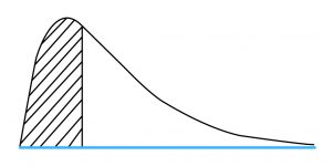
The chi-square distribution is asymmetrical and like the t-distribution, is a family of distributions. This means that a different distribution exists for each possible value of degrees of freedom, n – 1. Since the variance is a squared term, the minimum value can only be 0. Hence, the chi-square distribution is bounded below by 0. The graph below shows the shape of a chi-square distribution:

L1-V1-38

$\rm H_0: \sigma^2 = {\sigma}^2_0 \ versus \ H_a: \sigma^2 \neq {\sigma}^2_0.$ This is used when we believe the population variance is not equal to 0, or it is different from the hypothesized variance. It is a two-tailed test.
$\rm H_0: \sigma^2 \geq {\sigma}^2_0 \ versus \ H_a: \sigma^2 < {\sigma}^2_0.$ This is used when we believe the population variance is less than the hypothesized variance. It is a one-tailed test.
$\rm H_0: \sigma^2 \leq {\sigma}^2_0 \ versus \ H_a: \sigma^2 > {\sigma}^2_0.$ This is used when we believe the population variance is greater than the hypothesized variance. It is a one-tailed test.

After drawing a random sample from a normally distributed population, we calculate the test statistic using the following formula using n – 1 degrees of freedom:

where:

n = sample size

s = sample variance

We then determine the critical values using the level of significance and degrees of freedom. The chi-square distribution table is used to calculate the critical value.

Example

Consider Fund Alpha which we discussed in an earlier example. This fund has been in existence for 20 months. During this period the standard deviation of monthly returns was 5%. You want to test a claim by the fund manager that the standard deviation of monthly returns is less than 6%.

Solution:

The null and alternate hypotheses are: H₀: σ² ≥ 36 versus H_a: σ² < 36

Note that the standard deviation is 6%. Since we are dealing with population variance, we will square this number to arrive at a variance of 36%.

We then calculate the value of the chi-square test statistic:

c² = (n – 1) s² / σ₀² = 19 x 25/36 = 13.19

Next, we determine the rejection point based on df = 19 and significance = 0.05. Using the chi-square table, we find that this number is 10.117.

Since the test statistic (13.19) is higher than the rejection point (10.117) we cannot reject H₀. In other words, the sample standard deviation is not small enough to validate the fund manager’s claim that population standard deviation is less than 6%.

12.2 Test Concerning the Equality of Two Variances (F-Test)

In order to test the equality or inequality of two variances, we use an F-test which is the ratio of sample variances.

The assumptions for a F-test to be valid are:

The samples must be independent.
The populations from which the samples are taken are normally distributed.

Properties of the F-distribution

The F-distribution, like the chi-square distribution, is a family of asymmetrical distributions bounded from below by 0. Each F-distribution is defined by two values of degrees of freedom, called the numerator and denominator degrees of freedom. As shown in the figure below, the F-distribution is skewed to the right and is truncated at zero on the left hand side.

As shown in the graph, the rejection region is always in the right side tail of the distribution.

When working with F-tests, there are three hypotheses that can be formulated:

$\rm H_0 : \sigma_{12} = \sigma_{22} \ versus \ H_a: \sigma_{12} \neq \sigma_{22}$ . This is used when we believe the two population variances are not equal.
$\rm H_0 : \sigma_{12} \leq \sigma_{22} \ versus \ H_a: \sigma_{12} > \sigma_{22}$ . This is used when we believe the variance of the first population is greater than the variance of the second population.
$\rm H_0 : \sigma_{12} \geq \sigma_{22} \ versus \ H_a: \sigma_{12} < \sigma_{22}$ . This is used when we believe the variance of the first population is less than the variance of the second population.

The term σ₁²represents the population variance of the first population and σ₂²represents the population variance of the second population.

The formula for the test statistic of the F-test is:

$\rm F = \frac{{s_1}^2}{{s_2}^2}$

where:

$\rm {s_1}^2$ = the sample variance of the first population with n observations

$\rm {s_2}^2$ = the sample variance of the second population with n observations

A convention is to put the larger sample variance in the numerator and the smaller sample variance in the denominator.

df₁ = n₁ – 1 numerator degrees of freedom

df₂ = n₂ – 1 denominator degrees of freedom

The test statistic is then compared with the critical values found using the two degrees of freedom and the F-tables.

Finally, a decision is made whether to reject or not to reject the null hypothesis.

Example

You are investigating whether the population variance of the Indian equity market changed after the deregulation of 1991. You collect 120 months of data before and after deregulation.

Variance of returns before deregulation was 13. Variance of returns after deregulation was 18. Check your hypothesis at a confidence level of 99%.

Solution:

Null and alternate hypothesis: H₀: σ₁² = σ₂²versus H_A: σ₁² ≠ σ₂²

$\rm F-statistic: \frac{18}{13} = 1.4$

df = 119 for the numerator and denominator

α = 0.01 which means 0.005 in each tail. From the F-table: critical value = 1.6

Since the F-stat is less than the critical value, do not reject the null hypothesis.

13. Parametric vs. Nonparametric Tests

The hypothesis-testing procedures we have discussed so far have two characteristics in common:

They are concerned with parameters, such as the mean and variance.
Their validity depends on a set of assumptions.

Any procedure which has either of the two characteristics is known as a parametric test.

Nonparametric tests are not concerned with a parameter and/or make few assumptions about the population from which the sample are drawn. We use nonparametric procedures in three situations:

Data does not meet distributional assumptions.
Data has outliers
Data are given in ranks. (Example: relative size of the company and use of derivatives.)
The hypothesis does not concern a parameter. (Example: Is a sample random or not?)

14. Tests Concerning Correlation

The strength of linear relationship between two variables is assessed through correlation coefficient. The significance of a correlation coefficient is tested by using hypothesis tests concerning correlation.

There are two hypotheses that can be formulated (ρ represents the population correlation coefficient):

$H_0:\ \rho$ = 0

$H_a:\ \rho \neq$ 0

This test is used when we believe the population correlation is not equal to 0, or it is different from the hypothesized correlation. It is a two-tailed test.

14.1 Parametric Test of a Correlation

As long as the two variables are distributed normally, we can use sample correlation, r for our hypothesis testing. The formula for the t-test is

t = $\frac{r\ \sqrt{n-2}}{\sqrt{1-\ r^2}}$

where: n – 2 = degrees of freedom if H₀ is true.

The magnitude of r needed to reject the null hypothesis H₀: ρ= 0 decreases as sample size n increases due to the following:

As n increases, the number of degrees of freedom increases and the absolute value of the critical value t_c decreases.
As n increases, the absolute value of the numerator increases, leading to larger-magnitude t-values.

In other words, as n increases, the probability of Type-II error decreases, all else equal.

Example

The sample correlation between the oil prices and monthly returns of energy stocks in a Country A is 0.7986 for the period from January 2014 through December 2018. Can we reject a null hypothesis that the underlying or population correlation equals 0 at the 0.05 level of significance?

Solution:

$H_0:\ \rho$ = 0 –> true correlation in the population is 0.

$H_a:\ \rho \neq$ 0 –> correlation in the population is different from 0.

From January 2014 through December 2018, there are 60 months, so n = 60. We use the following statistic to test the above.

t = $\frac{0.7986\ \sqrt{60-2}}{\sqrt{1-\ {0.7986}^2}}$ = $\frac{6.0820}{0.6019}$ =10.1052

At the 0.05 significance level, the critical level for this test statistic is 2.00 (n = 60, degrees of freedom = 58). When the test statistic is either larger than 2.00 or smaller than 2.00, we can reject the hypothesis that the correlation in the population is 0. The test statistic is 10.1052, so we can reject the null hypothesis.

14.2 Tests Concerning Correlation: The Spearman Rank Correlation Coefficient

The Spearman rank correlation coefficient is equivalent to the usual correlation coefficient but is calculated on the ranks of two variables within their respective samples.

15. Test of Independence Using Contingency Table Data

A chi-square distributed test statistic is used to test for independence of two categorical variables. This nonparametric test compares actual frequencies with those expected on the basis of independence.

The test statistic is calculated as:

${\rm \chi }^{2}$ = $\sum _{i=1}^{m}\frac{\left(O_{ij} -E_{ij} \right)^{2} }{E_{ij} }$

where:

$$E_{ij}$ = $\frac{({\rm Total\; row\; }i)\times ({\rm Total\; column\; }j)}{{\rm Overall\; total}}$

This test statistic has degrees of freedom of (r − 1)(c − 2), where r is the number of categories for the first variable and c is the number of categories of the second variable.