
Shortfall risk
Shortfall risk is the risk that portfolio’s return will fall below a specified minimum level of return over a given period of time.
Safety first ratio
Safety first ratio is used to measure shortfall risk. It is calculated as:
![\rm SF-Ratio = \frac{[R_P \ - \ R_L]}{\sigma_P}](https://ift.world/wp-content/ql-cache/quicklatex.com-ee4de92982713ba71c7d02ec29b878b4_l3.png "Rendered by QuickLaTeX.com")
where:
Rp = Expected portfolio return
RL = Threshold level
 = Standard deviation of portfolio returns
The portfolio with the highest SF-Ratio is preferred, as it has the lowest probability of falling below the target return.
Example
An investor is considering two portfolios A and B. Portfolio A has an expected return of 10% and a standard deviation of 2%. Portfolio B has an expected return of 15% and a standard deviation of 10%. The minimum acceptable return for the investor is 8%. According to Roy’s safety first criteria, which portfolio should the investor select?
Solution:


Since A has a higher safety first ratio, the investor should select portfolio A.
Roy’s safety first criteria
It states that an optimal portfolio minimizes the probability that the actual portfolio return will fall below the target return.
If x is a random variable that is normally distributed, then to create a lognormal distribution of x we take ex and plot the values on a graph.
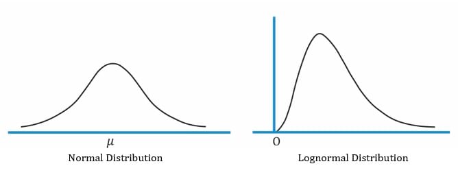
The properties of a lognormal distribution are:
Instructor’s Note: A normal distribution is more suitable as a model for returns than for asset prices, because returns generally vary about the mean, with a high probability of returns being close to the mean.
However, asset prices do not vary equally about a mean price, since the probability of extreme changes in price decreases as the price approaches zero. This means asset prices will not form a symmetrical graph like that of the normal distribution. Instead, asset prices follow a lognormal distribution, which is skewed to the right and cannot be negative.
Discretely compounded rates of returns have defined compounding periods such as quarterly, monthly etc. As we decrease the length of the compounding period, the effective annual rate rises. For continuous compounding, the EAR is given by:
EAR = er – 1
If we are given the holding period return over any time period, we can calculate the equivalent continuously compounded rate of return for that period as:
r = ln (HPR +1)
Example
If the holding period return of a stock was 10% for a period of one year. What is the equivalent continuously compounded rate of return for the year?
Solution:
r = ln (0.1 +1) = 0.0953 = 9.53%
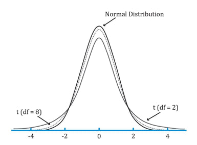
The Student’s t, chi-square, and F-distributions are mostly used to support statistical analyses, such as sampling, testing the statistical significance of estimated model parameters, or hypothesis testing.
The properties of a Student’s t-distribution are:
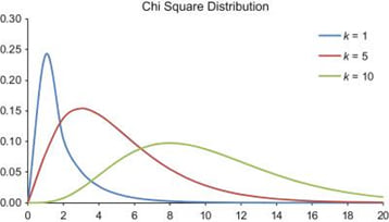
The properties of the Chi-square distribution are:
The properties of the F-distribution are:
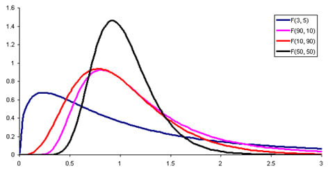
The relationship between the chi-square and F-distributions is as follows: If is one chi-square random variable with m degrees of freedom and is another chi-square random variable with n degrees of freedom, then  follows an F-distribution with m numerator and n denominator degrees of freedom.
Monte Carlo simulation is a computer simulation used to simulate possible security prices based on risk factors. As input, it uses randomly generated values for risk factors based on their assumed distributions. It processes this information as per the specified model and runs thousands of iterations. Then it gives the distribution of the expected value of the security as output.
Major applications include:
Limitations include:


Ace the Exam with Active Learning!

Ace the Exam with IFT Notes!
 Do IFT Mocks to make you exam-ready!

Accelerate your studies!

Practice your way to success!


Sign up to get more!