
In nearly all investment decisions, we work with random variables. To make probability statements about a random variable, we need to understand its probability distribution. A probability distribution specifies the probabilities of all possible outcomes of a random variable. In this reading, we will look at the following seven probability distributions:
A random variable is a variable whose outcome cannot be predicted. There are two basic types of random variables:
Probability distribution specifies the probabilities of all the possible outcomes for a random variable.
A cumulative distribution function defines the probability that a random variable, X, takes on a value equal to or less than a specific value, x. It is denoted as: F(x) = P(X ≤ x). It represents the sum of the probabilities for the outcomes up to and including a specified outcome.
The Discrete Uniform Distribution
The discrete uniform distribution has a finite number of specified outcomes and each outcome is equally likely. Consider a roll of a dice. The outcome is a random variable and it can take a value of 1 to 6. The probability that the random variable takes on any of these values is the same for all outcomes. With six outcomes, p(x) = 1/6 for all values of X (X = 1, 2, 3, 4, 5, 6). The table below summarizes the two views of this random variable – the probability function and the cumulative distribution function.
| X = x | Probability Function p(x) = P(X = x) | Cumulative Distribution Function F(x) = P(X ≤ x) |
| 1 | 1/6 | 1/6 |
| 2 | 1/6 | 2/6 |
| 3 | 1/6 | 3/6 |
| 4 | 1/6 | 4/6 |
| 5 | 1/6 | 5/6 |
| 6 | 1/6 | 6/6 |
Example
Using the table above, find the following probabilities:
Solution to 1:
To find F(4), we must find the cumulative probability of P(X ≤ 4) using the cumulative distribution function (third column). From the table, we can see that P(X ≤ 4) = 4/6 = 2/3. Therefore, the probability is 2/3.
Solution to 2:
To find P (3 ≤ X < 6), we need to find the sum of three probabilities: p(3), p(4), p(5). This is 1/6 + 1/6 + 1/6 = 3/6 = 1/2.
Solution to 3:
To find F(9), we must find the cumulative probability of P(X ≤ 9). This includes all possible outcomes, hence the probability is 1.
The continuous uniform distribution is defined over a range from a lower limit ‘a’ to an upper limit ‘b’. These limits serve as the parameters of the distribution.
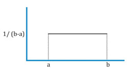
The probability that the random variable will take a value between x1 and x2, where x1 and x2 both lie within the range is given by:

Example
X is a uniformly distributed continuous random variable between 10 and 20. Calculate the probability that X will fall between 12 and 18.
Solution:
 = 0.6
= 0.6
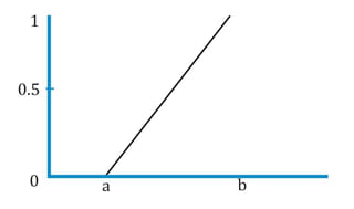
The cumulative distribution function for a continuous random variable is shown below:
Example
A commodity analyst predicts that the price per ounce of gold three years from now will be between $1,500 and $1,700. Assume gold prices follow a continuous uniform distribution. What is the probability that the price will be less than $1,600 three years from now?
Solution:
F(1,600) =  = 50% The probability that gold price will be less than $1,600 per ounce three years from now is 50%.
The building block of the binomial distribution is the Bernoulli random variable. A Bernoulli trial is one where there are only two possible outcomes: success or failure. Flipping a coin is an example of a Bernoulli trial – you either get heads or tails, but nothing else. This can be expressed as:
P (Y = 1) = p
P (Y = 0) = 1 – p
where:
p = probability that the trial is a success
In a binomial distribution, the random variable, X, is the number of successes in a given number of Bernoulli trials. Continuing with the coin example, say we flip the coin 10 times and we define success as ‘Heads’. Clearly with 10 flips we can get 0 to 10 successes.
The probability distribution of a binomial random variable for the probability of “x” success in “n” trials is calculated using the following formula:

where:
p = the probability of success on each trial
x = number of successes
n = number of trials
Instructor’s Note:
Two important points help illustrate the intuition behind the formula:
Example
If we flip a fair coin (p = 0.5) ten times (n = 10), what is the probability of seven successes?
Solution:
P(7) = P (X = 7) = 10C7 0.57 0.53 = 0.117
Mean and variance of a binomial variable
The mean and variance of a binomial variable can be calculated as:
| Random Variable | Mean | Variance |
| Bernoulli, B (1, p) | p | p (1 – p) |
| Binomial, B (n, p) | np | np (1 – p) |
For our coin-flip example, the mean value of the binomial random variable is np = 10 x 0.5 = 5. The intuition: if we perform the binomial experiment several times, where each experiment refers to 10 coin-flips, on average we will have 5 successes. The actual number of successes will be distributed equally on either side of the mean value. The random value for every trial moves closer to the expected value as the number of trials grows.
Example
Over the last 10 years, Abro corporation’s EPS increased year over year six times and decreased year over year four times. You decide to model the number of EPS increases for the next decade as a binomial random variable.
Solution to 1:
There are only two possible outcomes: increase in the EPS and no increase in the EPS.
Probability of success: p = 6/10 = 0.6
Probability of failure: 1 – p = 1 – 0.6 = 0.4
Solution to 2:
Using the binomial model:


Solution to 3:
Expected number of yearly EPS increases: 
Solution to 4:
Variance = 
Standard Deviation = 
The variance of the distribution is calculated as n p (1 – p) = 10 x 0.5 x (1 – 0.5) = 2.5
Binomial tree
A binomial tree can be used to model stock price movements. Refer to the tree diagram below. ‘S’ represents the initial stock price. ‘u’ represents an up move and ‘d’ represents a down move. The nodes show each possible value of the stock after 1, 2 and 3 time periods.
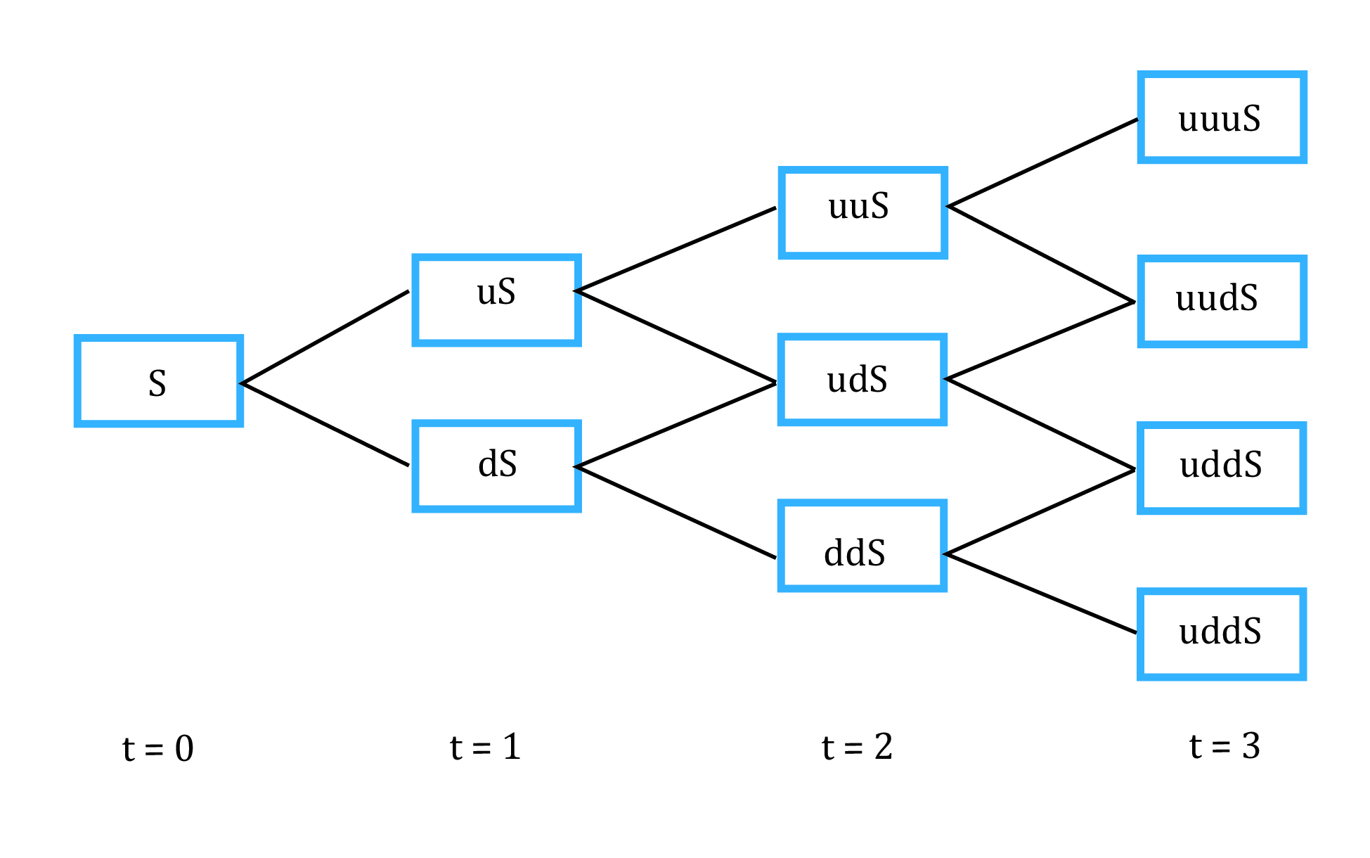
The expected stock price after each period is equal to the sum of possible stock prices at the end of the period multiplied by their respective probabilities.
Example
Consider an initial stock price of $100. In one time period, the stock can either rise by a factor of 1.1 or go down by a factor of 1/1.1. In any given time period, the probability of an up move is 0.6 and the probability of a down move is 0.4. After two periods, what are the possible stock prices and their respective probabilities? What is the expected stock price?
Solution:
uuS = 1.1 x 1.1 x 100 = 121 with probability 0.6 x 0.6 = 0.36
udS = 1.1 x 1/1.1 x 100 = 100 with probability 0.6 x 0.4 = 0.24
duS = 1/1.1 x 1.1 x 100 = 100 with probability 0.4 x 0.6 = 0.24
ddS = 1/1.1 x 1/1.1 x 100 = 82.64 with probability 0.4 x 0.4 = 0.16
Expected stock price = 121 x 0.36 + 100 x 0.24 + 100 x 0.24 + 82.64 x 0.16 = $104.78


Ace the Exam with IFT Notes!

Ace the Exam with Active Learning!

Accelerate your studies!
 Do IFT Mocks to make you exam-ready!

Practice your way to success!


Sign up to get more!