
A ‘population’ is defined as all members of a specified group. A ‘parameter’ describes the characteristics of a population.
A ‘sample’ is a subset drawn from a population. A ‘sample statistic’ describes the characteristic of a sample.
For example, all stocks listed on a country’s exchange refers to a population. If 30 stocks are selected from the listed stocks, then this refers to a sample.
Sample statistics—such as measures of central tendency, measures of dispersion, skewness, and kurtosis—help make probabilistic statements about investment returns.
Measures of central tendency specify where data are centered.
Measures of location include not only measures of central tendency but other measures that explain the location or distribution of data.
The arithmetic mean is the sum of the observations divided by the number of observations. It is the most frequently used measure of the middle or center of data.
The Sample Mean
The sample mean is the arithmetic mean calculated for a sample. It is expressed as:

where: n is the number of observations in the sample.
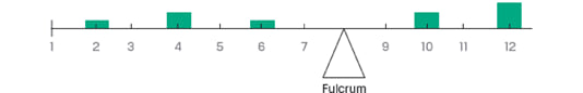
If the sample data is: 2, 4, 4, 6, 10, 10, 12, 12, and 12 the sample mean can be calculated as:

Properties of the Arithmetic Mean
The arithmetic mean can be thought of as the center of gravity of an object. Exhibit 36 from the curriculum illustrates this concept by the above observations on a bar. When the bar is placed on a fulcrum and the fulcrum is located at the arithmetic mean, the bar balances. At any other point the bar will not balance.
A drawback of the arithmetic mean is that it is sensitive to extreme values (outliers). It can be pulled sharply upward or downward by extremely large or small observations, respectively.
Outliers
When data contains outliers, there are three options to deal with the extreme values:
Option 1: Do nothing; use the data without any adjustment.
Option 2: Delete all the outliers.
Option 3: Replace the outliers with another value.
Option 1 is appropriate in cases when the extreme values are genuine.
Option 2 excludes extreme observations. A trimmed mean excludes a stated percentage of the lowest and highest values and then calculates the arithmetic mean of the remaining values. For example, a 5% trimmed mean discards the lowest 2.5% and the highest 2.5% of values and computes the mean of the remaining 95% of values.
Option 3 replaces extreme observations with observations closest to them. A winsorized mean assigns a stated percentage of the lowest values equal to one specified low value and a stated percentage of the highest values equal to one specified high value, and then computes a mean from the restated data. For example, a 95% winsorized mean sets the bottom 2.5% of values equal to the value at or below which 2.5% of all the values lie (the “2.5th percentile” value) and the top 2.5% of values equal to the value at or below which 97.5% of all the values lie (the “97.5th percentile” value).
The median is the midpoint of a data set that has been sorted into ascending or descending order.
For odd number of observations: 2,5,7,11,14 🡪 Median = 7
For even number of observations: 3, 9, 10, 20 🡪 Median = (9 + 10)/2 = 9.5
As compared to a mean, a median is less affected by extreme values (outliers).
The mode is the most frequently occurring value in a distribution.
For the following data set: 2, 4, 5, 5, 7, 8, 8, 8, 10, 12 🡪 Mode = 8
A distribution can have more than one mode, or even no mode. When a distribution has one mode it is said to be unimodal. If a distribution has two or three modes, it is called bimodal or trimodal respectively.
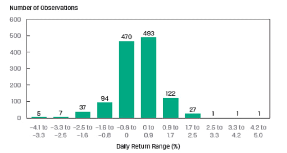
When working with continuous data such as stock returns, ‘modal interval’ is often used instead of a mode. The data is divided into bins and the bin with the highest frequency is considered the modal interval. Exhibit 39 from the curriculum demonstrates this concept by plotting a histogram of the daily returns on an index. The highest bar in the histogram ‘0.0 to 0.9%’ is the modal interval.
The Weighted Mean
In a weighted mean, instead of each data point contributing equally to the final mean, some data points contribute more “weight” than others. The formula for the weighted mean is:

where: the sum of the weights equals 1; that is 
Example
Consider an investor with a portfolio of three stocks. $40 is invested in A, $60 in B, and $100 in C. If returns were 5% on A, 7% on B, and 9% on C, compute the portfolio return using the weighted mean.
Solution:

Example:
A portfolio manager wishes to compute the weighted mean of a portfolio that has the following asset allocation:
| Local Equities: | 25% |
| International Equities: | 13% |
| Bonds: | 27% |
| Mortgage: | 18% |
| Gold: | 17% |
The returns on the above mentioned assets on December 31, 2012, were 5.4%, 8.9%, -2.5%, -7%, 11% respectively. What is the weighted mean for the portfolio?
Solution:
Weighted mean = (0.25 x 5.4) + (0.13 x 8.9) + (0.27 x -2.5) + (0.18 x -7) + (0.17 x 11) = 2.44%
An arithmetic mean is a special case of a weighted mean where all observations are equally weighted by the factor 1/n.
The Geometric Mean
The geometric mean is calculated as the nth root of a product of n numbers. The most common application of the geometric mean is to calculate the average return of an investment. The formula is:
![R_G={\left[\left(1\ +\ R_1\right)\left(1\ +\ R_2\right)\dots \left(1\ +\ R_n\right)\right]}^{\frac{1}{n}}\ -\ 1](https://ift.world/wp-content/ql-cache/quicklatex.com-e11c89f8704aebeb9c9e9d689d437cf8_l3.png "Rendered by QuickLaTeX.com")
Example
The return over the last four periods for a given stock is: 10%, 8%, -5% and 2%. Calculate the geometric mean.
Solution:
![{\left[\left(1\ +\ 0.10\right)\left(1\ +\ 0.08\right)\left(1\ -\ 0.05\right)\left(1\ +\ 0.02\right)\right]}^{\frac{1}{4}}-\ 1\ =\ 0.0358\ =\ 3.58\%](https://ift.world/wp-content/ql-cache/quicklatex.com-a01f45a60fbad1153f2f9edb862863a0_l3.png "Rendered by QuickLaTeX.com")
Given the returns shown above, $1 invested at the start of period 1 grew to:
$1.00 x 1.10 x 1.08 x 0.95 x 1.02 =$1.151. If the investment had grown at 3.58% every period, $1.00 invested at the start of period 1 would have increased to: $1.00 x 1.0358 x 1.0358 x 1.0358 x 1.0358 =$1.151 . As expected, both scenarios give the same answer. 3.58% is simply the average growth rate per period.
Other applications of the geometric mean involve the use of a second formula:

Instructor’s Note: This formula is less testable.
Example:
The P/E ratio of a stock over the past four years has been: 10, 15, 14, 13. Calculate the geometric mean P/E.
Solution:


Using Geometric and Arithmetic Means
The geometric mean is appropriate to measure past performance over multiple periods.
Example
The portfolio returns for the past two years were 100% in year 1 and -50% in year 2. What was the mean return?
Solution:
Past return = geometric mean = (2 x 0.5)0.5 – 1 = 0%
The arithmetic mean is appropriate for forecasting single period returns.
Example
Two possible returns for the next year are 100% and -50%. What is the expected return?
Solution:
Expected return = Arithmetic mean = (100 – 50)/2 = 25%
The Harmonic Mean
The harmonic mean is a special type of weighted mean in which an observation’s weight is inversely proportional to its magnitude. The formula for a harmonic mean is:

where:  > 0 for i = 1, 2,…n, and n is the number of observations
The harmonic mean is used to find average purchase price for equal periodic investments.
Example
An investor purchases $1,000 of a security each month for three months. The share prices are $10, $15 and $20 at the three purchase dates. Calculate the average purchase price per share for the security purchased.
Solution:
The average purchase price is simply the harmonic mean of $10, $15 and $20.
The harmonic mean is:

A more intuitive way of solving this is total money spent purchasing the shares divided by the total number of shares purchased.
Total money spent purchasing the shares = $1,000 x 3 = $3,000
Total shares purchased = sum of shares bought each month

= 100 + 66.67 + 50 = 216.67
Average purchase price per share = 
Comparison of AM, GM and HM
Which mean to use?


Ace the Exam with IFT Notes!

Ace the Exam with Active Learning!
 Do IFT Mocks to make you exam-ready!

Practice your way to success!

Accelerate your studies!


Sign up to get more!