LM02 Organizing, Visualizing, and Describing Data

Part 6

11. The Shape of the Distributions

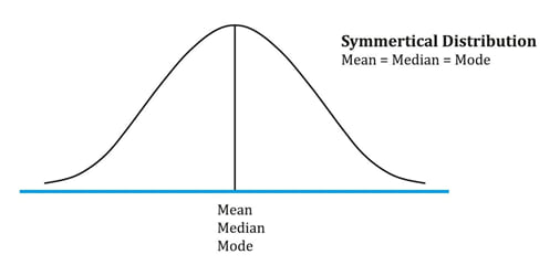
Symmetrical distribution

A distribution is said to be symmetrical when the distribution on either side of the mean is a mirror image of the other.

In a normal distribution, mean = median = mode.

If a distribution is non-symmetrical, it is said to be skewed. Skewness is a measure of the asymmetry of the probability distribution. Skewness can be negative or positive.

Positively skewed distribution

A positively skewed distribution has a long tail on the right side, which means that there will be limited but frequent downside returns and unlimited but less frequent upside returns.

Here the mean > median > mode. The extreme values affect the mean the most which is pulled to the right. They affect the mode the least.

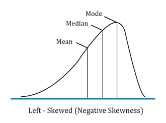
Negatively skewed distribution

A negatively skewed distribution has a long tail on the left side, which means that there will be limited but frequent upside returns and unlimited but less frequent downside returns.

Here the mean < median< mode. The extreme values affect the mean the most which is pulled to the left. They affect the mode the least.

Instructor’s Note: Investors prefer positive skewness because it has a higher chance of very large returns and also because it has a higher mean return.

Example:

Which of the following distribution is most likely characterized by frequent small losses and a few extreme gains?

1. Normal distribution
2. Negatively skewed
3. Positively skewed

Solution:

C is correct. A positively skewed distribution is characterized by frequent small losses and a few extreme gains.

Example:

Which of the following is most likely to be true for a negatively skewed distribution?

1. Mean < Median < Mode
2. Mode < Median < Mean
3. Median < Mean < Mode

Solution:

A is correct. In a negatively skewed distribution, the mean < median < mode.

11.1 The Shape of the Distributions: Kurtosis

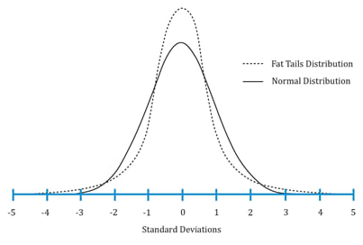
Kurtosis is a measure of the combined weight of the tails of a distribution relative to the rest of the distribution.

Excess kurtosis = kurtosis – 3. An excess kurtosis with an absolute value greater than one is considered significant.

• A leptokurtic distribution has fatter tails than a normal distribution. It has an excess kurtosis greater than 0.
• A platykurtic distribution has thinner tails than a normal distribution. It has an excess kurtosis less than 0.
• A mesokurtic distribution is identical to a normal distribution. It has an excess kurtosis equal to 0.

The following figure shows a leptokurtic distribution. As compared to a normal distribution, a leptokurtic distribution is more likely to generate observations in the tail region. It is also more likely to generate observations near the mean. However, to have the total probabilities sum to 1, it will generate fewer observations in the remaining regions (i.e. regions between the central and the two tail regions)

12. Correlation Between Two Variables

Covariance

Covariance is a measure of how two variables move together. The formula for computing the sample covariance of X and Y is:

The problem with covariance is that it can vary from negative infinity to positive infinity which makes it difficult to interpret. To address this problem, we use another measure called correlation.

Correlation

Correlation is a standardized measure of the linear relationship between two variables with values ranging between -1 and +1.

The sample correlation coefficient can be calculated as:

12.1 Properties of Correlation

• Correlation ranges from -1 and +1.
• A correlation of 0 (uncorrelated variables) indicates an absence of any linear (straight-line) relationship between the variables.
• A correlation of +1 indicates a perfect positive relationship.
• A correlation of -1 indicates a perfect negative relationship.

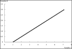
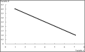
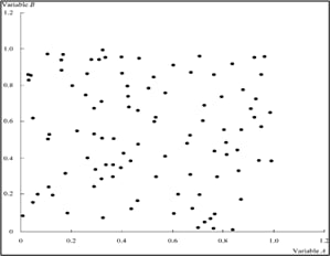
The three scatter plots below show a positive linear, negative linear, and no linear relation between two variables A and B. They have correlation coefficients of +1, -1 and 0 respectively.

Variables with a correlation of 1.

12.2 Limitations of Correlation Analysis

The correlation analysis has certain limitations:

• Two variables can have a strong non-linear relation and still have a very low correlation.
• The correlation can be unreliable when outliers are present.
• The correlation may be spurious. Spurious correlation refers to the following situations:
  • The correlation between two variables that reflects chance relationships in a particular data set.
  • The correlation induced by a calculation that mixes each of two variables with a third variable.
  • The correlation between two variables arising not from a direct relation between them, but from their relation to a third variable. Ex: shoe size and vocabulary of school children. The third variable is age here. Older shoe sizes simply imply that they belong to older children who have a better vocabulary.

Share on :