Exact matches only

Search in title

Search in content

Filter by Categories

101 concepts level I

101 concepts level II

2021 Level I Corporate Finance Full Videos

2021 Level I Economics Full Videos

2021 Level I Ethics Full Videos

2021 Level I FRA Full Videos

2021 Level I Portfolio Management Full Videos

2021 Level I Quantitative Methods Full Videos

Advice and How to Study Videos

All-Levels

Alternative Investments

Alternative Investments (AI)

BookLet Top Level

Corporate Issuers

Corporate Issuers (CI)

Demystified Videos

Derivatives

Derivatives (DV)

Economics

Economics (EC)

Equity

Equity Investments (EI)

Ethical and Professional Standards (ES)

Ethics

featured

Financial Reporting and Analysis

Financial Statement Analysis (FSA)

Fixed Income

Fixed Income (FI)

Level I

Level II

Level III

LM01 Alternative Investment Features, Methods, and Structures

LM01 Categories, Characteristics, and Compensation Structures of Alternative Investments

LM01 Corporate Structures and Ownership

LM01 Derivative Instrument and Derivative Market Features

LM01 Ethics and Trust in the Investment Profession

LM01 Fixed-Income Instrument Features

LM01 Fixed-Income Securities: Defining Elements

LM01 Introduction to Financial Statement Analysis

LM01 Market Organization & Structure

LM01 Market Organization and Structure

LM01 Organizational Forms, Corporate Issuer Features, and Ownership

LM01 Portfolio Management Overview

LM01 Portfolio Management: An Overview

LM01 Rates and Returns

LM01 The Firm & Market Structures

LM01 Time Value of Money

LM01 Topics in Demand and Supply Analysis

LM02 Alternative Investment Performance and Returns

LM02 Analyzing Income Statements

LM02 Code of Ethics and Standards of Professional Conduct

LM02 Code of Ethics and Standards of Professional Conduct Profession

LM02 Financial Reporting Standards

LM02 Fixed Income Markets - Issuance Trading and Funding

LM02 Fixed-Income Cash Flows and Types

LM02 Forward Commitment and Contingent Claim Features and Instruments

LM02 Introduction to Corporate Governance and Other ESG Considerations

LM02 Investors and Other Stakeholders

LM02 Organizing, Visualizing, and Describing Data

LM02 Performance Calculation and Appraisal of Alternative Investments

LM02 Portfolio Risk & Return: Part I

LM02 Portfolio Risk and Return Part I

LM02 Security Market Indexes

LM02 The Firm and Market Structures

LM02 Time Value of Money in Finance

LM02 Understanding Business Cycles

LM03 Aggregate Output, Prices and Economic Growth

LM03 Analyzing Balance Sheets

LM03 Business Models & Risks

LM03 Corporate Governance: Conflicts, Mechanisms, Risks, and Benefits

LM03 Derivative Benefits, Risks, and Issuer and Investor Uses

LM03 Fiscal Policy

LM03 Fixed-Income Issuance and Trading

LM03 Guidance for Standards I-VII

LM03 Guidance for Standards I–VII

LM03 Introduction to Fixed Income Valuation

LM03 Investments in Private Capital: Equity and Debt

LM03 Market Efficiency

LM03 Portfolio Risk & Return: Part II

LM03 Portfolio Risk and Return Part II

LM03 Private Capital, Real Estate, Infrastructure, Natural Resources, and Hedge Funds

LM03 Probability Concepts

LM03 Statistical Measures of Asset Returns

LM03 Understanding Income Statements

LM04 An Introduction to Asset-Backed Securities

LM04 Analyzing Statements of Cash Flows I

LM04 Arbitrage, Replication, and the Cost of Carry in Pricing Derivatives

LM04 Basics of Portfolio Planning & Construction

LM04 Basics of Portfolio Planning and Construction

LM04 Capital Investments

LM04 Common Probability Distributions

LM04 Fixed-Income Markets for Corporate Issuers

LM04 Introduction to the Global Investment Performance Standards (GIPS)

LM04 Monetary Policy

LM04 Overview of Equity Securities

LM04 Probability Trees and Conditional Expectations

LM04 Real Estate and Infrastructure

LM04 Understanding Balance Sheets

LM04 Understanding Business Cycles

LM04 Working Capital and Liquidity.

LM05 Analyzing Statements of Cash Flows II

LM05 Capital Investments and Capital Allocation

LM05 Company Analysis: Past and Present

LM05 Fixed-Income Markets for Government Issuers

LM05 Introduction to Geopolitics

LM05 Introduction to Industry and Company Analysis

LM05 Monetary and Fiscal Policy

LM05 Natural Resources

LM05 Portfolio Mathematics

LM05 Pricing and Valuation of Forward Contracts and for an Underlying with Varying Maturities

LM05 Pricing and Valuation of Forward Contracts.

LM05 Sampling and Estimation

LM05 The Behavioral Biases of Individuals

LM05 Understanding Cash Flow Statements

LM05 Understanding Fixed-Income Risk and Return

LM05 Working Capital & Liquidity

LM06 Analysis of Inventories

LM06 Capital Structure

LM06 Cost of Capital-Foundational Topics

LM06 Equity Valuation: Concepts and Basic Tools

LM06 Financial Analysis Techniques

LM06 Fixed-Income Bond Valuation: Prices and Yields

LM06 Fundamentals of Credit Analysis

LM06 Hedge Funds

LM06 Hypothesis Testing

LM06 Industry and Competitive Analysis

LM06 International Trade

LM06 Introduction to Geopolitics

LM06 Introduction to Risk Management

LM06 Pricing and Valuation of Futures Contracts

LM06 Simulation Methods

LM07 Analysis of Long-Term Assets

LM07 Business Models

LM07 Capital Flows and the FX Market

LM07 Capital Structure

LM07 Company Analysis: Forecasting

LM07 Estimation and Inference

LM07 International Trade and Capital Flows

LM07 Introduction to Digital Assets

LM07 Introduction to Linear Regression

LM07 Inventories

LM07 Pricing and Valuation of Interest Rate and Other Swaps

LM07 Pricing and Valuation of Interest Rates and Other Swaps

LM07 Technical Analysis

LM07 Yield and Yield Spread Measures for Fixed-Rate Bonds.

LM08 Currency Exchange Rates

LM08 Equity Valuation: Concepts and Basic Tools

LM08 Exchange Rate Calculations

LM08 Fintech in Investment Management

LM08 Hypothesis Testing

LM08 Long Lived Assets

LM08 Measures of Leverage

LM08 Pricing and Valuation of Options

LM08 Topics in Long-Term Liabilities and Equity

LM08 Yield and Yield Spread Measures for Floating-Rate Instruments

LM09 Analysis of Income Taxes

LM09 Income Taxes

LM09 Option Replication Using Put-Call Parity

LM09 Option Replication Using Put–Call Parity

LM09 Parametric and Non-Parametric Tests of Independence

LM09 The Term Structure of Interest Rates: Spot, Par, and Forward Curves

LM10 Financial Reporting Quality

LM10 Interest Rate Risk and Return

LM10 Non-current (Long-Term) Liabilities

LM10 Simple Linear Regression

LM10 Valuing a Derivative Using a One-Period Binomial Model

LM11 Financial Analysis Techniques

LM11 Financial Reporting Quality

LM11 Introduction to Big Data Techniques

LM11 Yield-Based Bond Duration Measures and Properties

LM12 Applications of Financial Statement Analysis

LM12 Introduction to Financial Statement Modeling

LM12 Yield-Based Bond Convexity and Portfolio Properties

LM13 Curve-Based and Empirical Fixed-Income Risk Measures

LM14 Credit Risk

LM15 Credit Analysis for Government Issuers

LM16 Credit Analysis for Corporate Issuers

LM17 Fixed-Income Securitization

LM18 Asset-Backed Security (ABS) Instrument and Market Features

LM19 Mortgage-Backed Security (MBS) Instrument and Market Features

New Booklet Top level

Portfolio Management

Portfolio Management (PM)

Quantitative Methods

Quantitative Methods (QM)

Uncategorized

Please select your exam.

IFT Notes for Level I CFA^® Program

LM02 Organizing, Visualizing, and Describing Data

Part 5

8. Quantiles

8.1 Quartiles, Quintiles, Deciles, and Percentiles

A quantile is a value at or below which a stated fraction of the data lies. Some examples of quantiles include:

Quartiles: The distribution is divided into quarters.
Quintiles: The distribution is divided into fifths.
Deciles: The distribution is divided into tenths.
Percentile: The distribution is divided into hundredths.

The formula for the position of a percentile in a data set with n observations sorted in ascending order is:

$L_y=\frac{\left(n\ +\ 1\right)y}{100}$

where:
y is the percentage point at which we are dividing the distribution.
n is the number of observations.
L_y is the location (L) of the percentile (P_y) in an array sorted in ascending order.

Some important points to remember are:

When the location, L_y, is a whole number, the location corresponds to an actual observation.
When L_y is not a whole number or integer, L_y lies between the two closest integer numbers (one above and one below) and we use linear interpolation between those two places to determine P_y.
Interquartile range is the difference between the third and the first quartiles.

Example

Consider the data set:

47 35 37 32 40 39 36 34 35 31 44

Find the 75^th percentile point
Find the 1^st quartile and 3^rd quartile
Calculate the interquartile range
Find the 5^th decile point
Find the 6^th decile point.

Solution to 1:

First arrange the data in ascending order:

31, 32, 34, 35, 35, 36, 37, 39, 40, 44, 47

Location of the 75^th percentile is the:
L₇₅ = (11 + 1) (75/100) = 9^th value. i.e. P₇₅= 40

With a small data set, such as this one, the location and the value is approximate. As the data set becomes larger, the location and percentile value estimates become more precise.

Solution to 2:

Location of the 1^st quartile is:

L₂₅ = (11 + 1) (25/100) = 3^rd value. i.e. P₂₅= 34

Location of the 3^rd quartile is:

L₇₅ = (11 + 1) (75/100) = 9^th value. i.e. P₇₅= 40

Solution to 3:

The interquartile range is the difference between the third and first quartiles, 40 – 34 = 6

Solution to 4:

Location of the 5th decile is:

L₅₀ = (11 + 1) (50/100) = 6^th value. i.e. P₅₀= 36

Solution to 5:

L₆₀ = (11 + 1) (60/100) = 7.2

Use linear interpolation, which estimates an unknown value on the basis of two known values that surround it.

In this case, the 7^th value is 37 and the 8^th value is 39. The 6^th decile is: P₆₀= 37+ 0.4 (0.2 times the linear distance between 37 and 39). P₆₀= 37.4

A box and whiskers plot is used to visualize the dispersion of data across quartiles. The box represents the interquartile range. The whiskers represent the highest and lowest values of the distribution. Exhibit 44 shows a sample box and whisker plot.

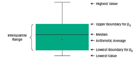
There are several variations of the box and whiskers plot. Sometimes the whiskers may be a function of the interquartile range instead of the highest and lowest values.

8.2 Quantiles in Investment Practice

Quantiles are used in:

Portfolio performance evaluation: The performance of investment managers is often evaluated in terms of the percentile or quartile in which they fall relative to the performance of their peers.
Investment research: For example, companies can be ranked based on their market capitalization and sorted into deciles. The first decile contains companies with smallest market values and the tenth decile contains companies with the largest market values. Such a classification allows analysts to compare the performance of small companies with large ones.

9. Measures of Dispersion

Measures of central tendency tell us where the investment results (expected returns) are centered. However, to evaluate an investment we also need to know how returns are dispersed around the mean. Measures of dispersion describe the variability of outcomes around the mean.

9.1 The Range

The range is the difference between the maximum and minimum values in a data set. It is expressed as:

Range = Max value – Min Value

If the annual returns data is: 10%, -5%, 10%, 25%. What is the range?

Here the maximum return is 25% and the minimum return is -5%. The range is 25% – (-5%) = 30%.

Another way to specify the range is to mention the actual minimum and maximum values. For example, for the above data the range is “from -5% to 25%”.

The range is easy to compute; however, it does not tell us much about how the data is distributed.

9.2 The Mean Absolute Deviation

It is the average of the absolute values of deviations from the mean. It is expressed as:

MAD= $\left[\sum^n_{i=1}{}\left|X_i-\ \overline{X}\right|\right]/n$

where: $\overline{X}$ is the sample mean and n is the number of observations in the sample.

Example

Consider the following data set: 8, 12, 10, 8 and 5. Calculate the mean absolute deviation.

Solution:

$\overline{X}$ = (8 + 12 + 10 + 8 + 5) / 5 = 8.6

$MAD=\frac{\left|8-8.6\right|+\left|12-8.6\right|+\left|10-8.6\right|+\left|8-8.6\right|+\left|5-8.6\right|}{5}$

$MAD=\frac{0.6\ +\ 3.4\ +\ 1.4\ +\ 0.6\ +\ 3.6}{5}=\ 1.92$

9.3 Sample Variance and Sample Standard Deviation

Variance is defined as the average of the squared deviations around the mean. Standard deviation is the positive square root of the variance.

Sample variance applies when we are dealing with a subset, or sample, of the total population. It is expressed as:

$s^2=\ \sum^n_{i=0}{}(X_i-\ \overline{X}\ ){\ }^2\ /\ (n-1)$

where: $\overline{X}$ is the sample mean and n is the number of observations in the sample.

Sample standard deviation is defined as the positive square root of the sample variance

$s^2=\frac{\left[{\left(8-8.6\right)}^2+{\left(12-8.6\right)}^2+{\left(10-8.6\right)}^2+{\left(8-8.6\right)}^2+{\left(5-8.6\right)}^2\right]}{5-1}$

$s^2=6.80\%$

The sample standard deviation is the positive square root of the sample variance. For the sample data given above, s= √6.80 = 2.61%

Using a financial calculator to calculate variance and standard deviations

The sample standard deviation can easily be computed using a financial calculator. Assume the following data set: 10%, -5%, 10%, 25%, the calculator key strokes are shown below:

Keystrokes	Description	Display
[2nd] [DATA]	Enters data entry mode
[2nd] [CLR WRK]	Clears data register	X01
10 [ENTER]		X01 = 10
[↓] [↓] 5+/- [ENTER]		X02 = -5
[↓] [↓] 10 [ENTER]		X03 = 10
[↓] [↓] 25 [ENTER]		X04 = 25
[2nd] [STAT] [ENTER]	Puts calculator into stats mode
[2nd] [SET]	Press repeatedly till you see 🡪	1-V
[↓]	Number of data points	N = 4
[↓]	Mean	X = 10
[↓]	Sample standard deviation	Sx = 12.25
[↓]	Population standard deviation	σx = 10.61

Notice that the calculator gives both the sample and the population standard deviation. On the exam we will have to determine whether we are dealing with population or sample data and choose the appropriate value.

Dispersion and the relationship between the arithmetic and the geometric means

The sample standard deviation can be used to understand the gap between the arithmetic and geometric mean. The relationship between the arithmetic mean ( $\overline{X}$ ) and geometric mean( $\overline{X_{G}}$ ) is:

${\overline{X}}_G\approx \overline{X}-\frac{s^2}{2}$

The larger the variance of the sample, the wider the difference between the geometric mean and the arithmetic mean.

Example:

The dividend yield for five hypothetical companies from a list of ten companies is given below. What is the sample variance?

Paknama	10.50%
Genie Ltd.	16.25%
Mirinda Corp.	27.00%
Tina Travels Ltd.	12.00%
Thomas Press Ltd.	7.80%

Solution:

$\overline{X}=\frac{10.5+16.25+27+12+7.8}{5}=14.71$

Sample variance= $\frac{[{\left(10.5-14.71\right)}^2+{\left(16.25-14.71\right)}^2+{\left(27-14.71\right)}^2+{\left(12-14.71\right)}^2{+\left(7.8-14.71\right)}^2]}{5-1}$

Sample variance = 56.49

10. Downside Deviation and Coefficient of Variation

Variance and standard deviation of returns take account of returns above and below the mean, but often investors are concerned only with downside risk, for example returns below the mean.

The target downside deviation, or target semideviation, is a measure of the risk of being below a given target. It is calculated as the square root of the average squared deviations from the target, but it includes only those observations below the target (B).

The sample target semideivation can be calculated as:

$S_{Target}=\sqrt{\sum^n_{for\ all\ X_i\le B}{}\frac{{(X_i-B)}^2}{n-1}}$

Example:

Suppose the monthly returns on a portfolio are as shown:

Month	Return (%)
Jan	6
Feb	4
Mar	-2
Apr	-5
May	5
Jun	2
Jul	1
Aug	0
Sep	4
Oct	3
Nov	0
Dec	2

Calculate the target downside deviation when the target return is 4%.

Solution:

Month	Observation	Deviation from the 4% target	Deviation below the target	Squared deviations below the target
Jan	6	2	–	–
Feb	4	0	–	–
Mar	-2	-6	-6	36
Apr	-5	-9	-9	81
May	5	1	–	–
Jun	2	-2	-2	4
Jul	1	-3	-3	9
Aug	0	-4	-4	16
Sep	4	0	–	–
Oct	3	-1	-1	1
Nov	0	-4	-4	16
Dec	2	-2	-2	4
Sum				167

$Target\ semideviation=\ \sqrt{\frac{167}{11}}=3.8964\%$

The target downside deviation will be less than the standard deviation, because deviations above the target are ignored. As the target is increased, the target downside deviation will increase.

10.1 Coefficient of Variation

Coefficient of variation expresses how much dispersion exists relative to the mean of a distribution and allows for direct comparison of dispersion across different data sets, even if the means are drastically different from one another. It is used in investment analysis to compare relative risks. When evaluating investments, a lower value is better. Coefficient of variation is expressed as:

$CV=\frac{s}{\overline{X}}$

where: s = sample standard deviation of a set of observations and $\overline{X}$ = sample mean

Example

Investment A has a mean return of 7% and a standard deviation of 5%. Investment B has a mean return of 12% and a standard deviation of 7%. Calculate the coefficients of variation.

Solution

The coefficients of variation can be calculated as follows:

${CV}_A=\frac{5\%}{7\%}=0.71$