
If the occurrence of one event does not influence the occurrence of the other event, then the two events are called independent events.
i.e. P(A|B) = P(A) or P(B|A) = P(B)
Multiplication rule for independent events: P(AB) = P(A) P(B)
Addition rule for independent events: P(A or B) = P(A) + P(B) – P(AB). (The addition rule does not change.)
If the probability of an event is affected by the occurrence of another event then it is called a dependent event.
The total probability rule is used to calculate the unconditional probability of an event, given conditional probabilities.
In investment analysis, we often formulate a set of mutually exclusive and exhaustive scenarios and then estimate the probability of a particular event. For example, let’s say that we have two scenarios S and non-S that are mutually exclusive and exhaustive.
According to the total probability rule, the probability of any event P(A) can be expressed as:
P(A) = P(AS) + P(ASC)
Using the multiplication rule we get,
P(A) = P(A|S) P(S) + P(A|SC) P(SC)
If we have more than two scenarios, we can generalize this equation to:
P(A) = P(AS1) + P(AS2) +… + P(ASn) = P(A|S1) P(S1) + P(A|S2) P(S2) + … + P(A|Sn) P(Sn)
The expected value of a random variable can be defined as the probability-weighted average of the possible outcomes of the random variable. For a random variable X, the expected value of X is denoted as E(X) and is calculated as:

where:
Xi = One of n possible outcomes of the random variable X
P(Xi) = Probability of Xi
The expected value is our forecast, but we cannot count on the individual forecast being realized. This is why we need to measure the risk we face. Variance and standard deviation are examples of how we can measure this risk. The variance of a random variable is the probability-weighted sum of the squared differences between each possible outcome and the expected value of the random variable. It is expressed as:
![{\sigma }^2\left(X\right)=\ \sum\limits_{i=1}^{n}{P\left(X\right)\ {\left[X-E\left(X\right)\right]}^2}](https://ift.world/wp-content/ql-cache/quicklatex.com-e93f5d2c396f12c0088d0b234c9cabd2_l3.png "Rendered by QuickLaTeX.com")
Variance is a number greater than or equal to 0 because it is the sum of squared terms. If variance is 0, there is no dispersion or risk. The outcome is certain and the quantity X is not random at all. Standard deviation is the positive square root of variance.
We can calculate the expected value and variance of a random variable using a financial calculator as shown below:
Example
A project’s cash flow for the upcoming year depends on the state of the economy, as shown in the table below. What is the variance of the cash flow? What is the standard deviation?
| State of Economy | Probability | Cash Flow |
| Good | 0.3 | 50 |
| Average | 0.5 | 40 |
| Weak | 0.2 | 20 |
Solution:
Using a financial calculator:
| Keystrokes | Explanation | Display |
| [2nd] [DATA] | Enters data entry mode | |
| [2nd] [CLR WRK] | Clears data register | X01 |
| 50 [ENTER] | 1st possible value of random variable | X01 = 50 |
| [↓] 30 [ENTER] | Probability of 30% for X01 | Y01 = 30 |
| [↓] 40 [ENTER] | 2nd possible value of random variable | X02 = 40 |
| [↓] 50 [ENTER] | Probability of 50% for X02 | Y02 = 50 |
| [↓] 20 [ENTER] | 3rd possible value of random variable | X03 = 20 |
| [↓] 20 [ENTER] | Probability of 20% for X03 | Y03 = 20 |
| [2nd] [STAT] | Puts calculator into stats mode | |
| [2nd] [SET] | Press repeatedly till you see à | 1-V |
| [↓] | Total number of entries | N = 100 |
| [↓] | Expected value of random variable | X = 39 |
| [↓] | Sample standard deviation | Sx = 10.49 |
| [↓] | Population standard deviation | σx = 10.44 |
We can then square the population standard deviation of 10.44 to get the variance i.e. 10.442 = 109.00
Just like the total probability rule states unconditional probabilities in terms of conditional probabilities, the total probability rule for expected values states unconditional expected values in terms of conditional expected values.
E(X|S) = P(X1|S) X1 + P(X2|S) X2 + … + P(Xn|S) Xn
Instructor’s Note
Notice that this formula is exactly similar to the total probability rule formula.
P(A) = P(A|S1) P(S1) + P(A|S2) P(S2) + … + P(A|Sn) P(Sn)
Example
What is the expected price of a stock at the end of the current period given the following information: probability that interest rates will decline = 0.4. If interest rates decline there is a 75% chance that stock price will be $100 versus a 25% chance that the stock price will be $90. If interest rates do not decline there is a 50% chance that the stock price will be $80 versus a 50% chance that stock price will be $70.
Solution:
We can plot the probabilities using a tree diagram.
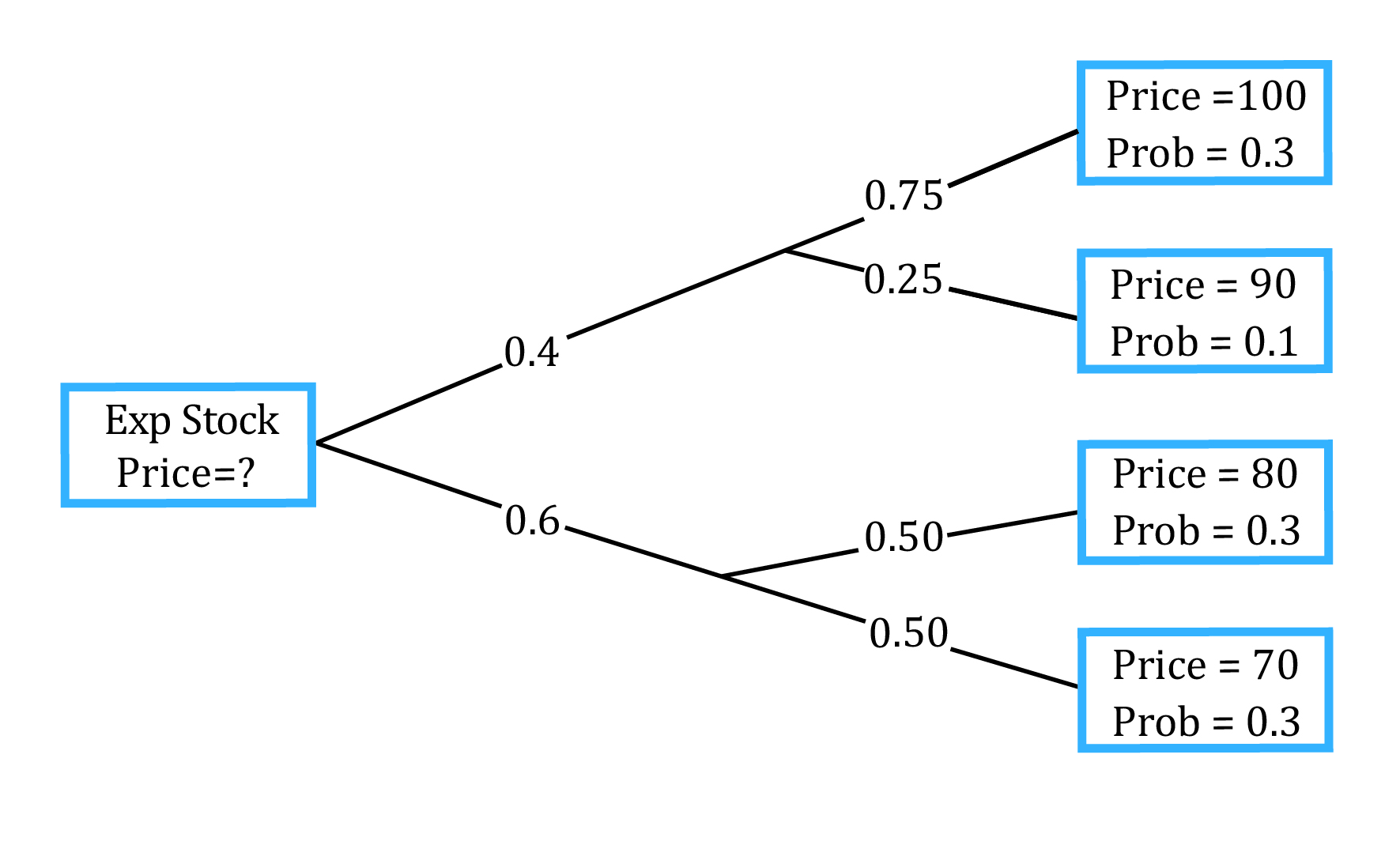
Consider the first node (top right). It refers to the probability that the stock price will be $100 given a decline in interest rates. We can calculate the probability of that happening by multiplying the probability of a decline in interest rates (0.4) by the probability of the stock price being $100 if that happens (0.75). This gives us a conditional probability of 0.30. In short, it is the joint probability of the stock price being $100 given a decline in interest rates. Similarly, probabilities are calculated for each of the other three nodes. We can then calculate:
E(Price│decline in interest rates) = 0.75 ($100) + 0.25 ($90) = $97.50
E(Price│no decline in interest rates) = 0.50 ($80) + 0.50 ($70) = $75.00
Now we use the total probability rule for expected value of stock price at the end of the current period:
E(Price) = E(Price│decline in interest rates) P(decline in interest rates) + E(Price│no decline in interest rates) P(no decline in interest rates)
E(Price) = $97.50 (0.40) + $75.00 (0.60)
E(Price) = $84.00


Ace the Exam with IFT Notes!

Ace the Exam with Active Learning!

Accelerate your studies!
 Do IFT Mocks to make you exam-ready!

Practice your way to success!


Sign up to get more!