
In reaching a statistical decision, we can make two possible errors:
The following table shows the possible outcomes of a test.
| Decision | True condition | |
| H0 true | H0 false | |
| Do not reject H0 | Correct decision | Type II error |
| Reject H0 (accept Ha) | Type I error | Correct decision |
The probability of a Type I error is also known as the level of significance of a test and is denoted by ‘α’. A related term, confidence level is calculated as (1 – α ). For example, a level of significance of 5% for a test means that there is a 5% probability of rejecting a true null hypothesis and corresponds to the 95% confidence level.
Controlling the two types of errors involves a trade-off. If we decrease the probability of a Type I error by specifying a smaller significance level (for e.g., 1% instead of 5%), we increase the probability of a Type II error. The only way to reduce both types of error simultaneously is by increasing the sample size, n.
The probability of a Type II error is denoted by ‘β’. The power of test is calculated as (1 – β). It represents the probability of correctly rejecting the null when it is false.
The different probabilities associated with the hypothesis testing decisions are presented in the table below:
| Decision | True condition | |
| H0 true | H0 false | |
| Do not reject H0 | Confidence level (1 – α ) | β |
| Reject H0 (accept Ha) | Level of significance (α) | Power of the test (1 – β) |
The most commonly used levels of significance are: 10%, 5% and 1%.
A decision rule involves determining the critical values based on the level of significance; and comparing the test statistic with the critical values to decide whether to reject or not reject the null hypothesis. When we reject the null hypothesis, the result is said to be statistically significant.
One-tailed test:
Continuing with our Asian stocks example, suppose we want to test if the population mean is greater than 2%. Say we want to test our hypothesis at the 5% significance level. This is a one-tailed test and we are only interested in the right tail of the distribution. (If we were trying to assess whether the population mean is less than 2%, we would be interested in the left tail.)
The critical value is also known as the rejection point for the test statistic. Graphically, this point separates the acceptance and rejection regions for a set of values of the test statistic. This is shown below:
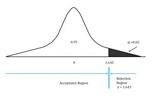
The region to the left of the test statistic is the ‘acceptance region’. This represents the set of values for which we do not reject (accept) the null hypothesis. The region to the right of the test statistic is known as the ‘rejection region’.
Using the Z –table and 5% level of significance, the critical value = Z0.05= 1.65
In a two-tailed test, two critical values exist, one positive and one negative. For a two-sided test at the 5% level of significance, we split the level of significance equally between the left and right tail i.e. (0.05/2) = 0.025 in each tail.
This corresponds to rejection points of +1.96 and -1.96. Therefore, we reject the null hypothesis if we find that the test statistic is less than -1.96 or greater than +1.96. We fail to reject the null hypothesis if -1.96 ≤ test statistic ≤ +1.96. Graphically, this can be shown as:
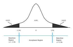
The above figure also illustrates the relationship between confidence intervals and hypothesis tests. A confidence interval specifies the range of values that may contain the hypothesized value of the population parameter. The 5% level of significance in the hypothesis tests corresponds to a 95% confidence interval. When the hypothesized value of the population parameter is outside the corresponding confidence interval, the null hypothesis is rejected. When the hypothesized value of the population parameter is inside the corresponding confidence interval, the null hypothesis is not rejected.
In this step we first ensure that the sampling procedure does not include biases, such as sample selection or time bias. Then, we cleanse the data by removing inaccuracies and other measurement errors in the data. Once we are convinced that the sample data is unbiased and accurate, we use it to calculate the appropriate test statistic.
A statistical decision simply consists of rejecting or not rejecting the null hypothesis.
If the test statistic lies in the rejection region, we will reject H0. On the other hand, if the test statistic lies in the acceptance region, then we cannot reject H0.
An economic decision takes into consideration all economic issues relevant to the decision, such as transaction costs, risk tolerance, and the impact on the existing portfolio. Sometimes a test may indicate a result that is statistically significant, but it may not be economically significant.
The p-value is the smallest level of significance at which the null hypothesis can be rejected. It can be used in the hypothesis testing framework as an alternative to using rejection points.
For example, if the p-value of a test is 4%, then the hypothesis can be rejected at the 5% level of significance, but not at the 1% level of significance.
Relationship between test-statistic and p-value
A high test-statistic implies a low p-value.
A low test-statistic implies a high p-value.
A Type I error represents a false positive result – rejecting the null when it is true. When multiple hypothesis tests are run on the same population, some tests will give false positive results. The expected portion of false positives is called the false discovery rate (FDR). For example, if you run 100 tests and use a 5% level of significance, you will get five false positives on average. This issue is called the multiple testing problem.
To overcome this issue, the false discovery approach is used to adjust the p-values when you run multiple tests. The researcher first ranks the p-values from the various tests from lowest to highest. He then makes the following comparison, starting with the lowest p-value (with k = 1), p(1):

This comparison is repeated until we find the highest ranked p(k) for which this condition holds. For example, say we perform this check for k=1, k=2, k=3, and k=4; and we find that the condition holds true for k=4. Then we can say that the first four tests ranked on the basis of the lowest p-values are significant.


Ace the Exam with Active Learning!

Ace the Exam with IFT Notes!

Accelerate your studies!
 Do IFT Mocks to make you exam-ready!

Practice your way to success!


Sign up to get more!