IFT Notes for Level I CFA^® Program

LM07 Introduction to Linear Regression

Part 2

5. Hypothesis Testing of Linear Regression Coefficients

5.1 Hypothesis Tests of the Slope Coefficient

In order to test whether an estimated slope coefficient is statistically significant, we use hypothesis testing.

Continuing with our previous example of a simple linear regression with ROA as the dependent variable and CAPEX as the independent variable. Suppose we want to test whether the slope coefficient of CAPEX is different from zero.

The steps are:

Step 1: State the hypothesis

H₀: b₁ = 0; H_a:b₁≠ 0

Step 2: Identify the appropriate test statistic

To test the significance of individual slope coefficients we use the t-statistic. It is calculated by subtracting the hypothesized population slope (B₁) from the estimated slope coefficient ( $\widehat{b_1}$ ) and then dividing this difference by the standard error of the slope coefficient, $s_{\widehat{b_1}}$ :

t= $\frac{\widehat{b_1}\ -\ B_1}{s_{\widehat{b_1}}}$ = $\frac{Estimated\ value-Hypothesized\ value}{standard\ error}$

with n – 2 = 6 – 2 = 4 degrees of freedom

Step 3: Specify the level of significance

Typically, a 5% level of significance is selected.

Step 4: State the decision rule

Since the alternate hypothesis contains a ‘≠’ sign, this is a two tailed test. For a 5% level of significance, 4 degrees of freedom and a two tailed test the critical t-values are ±2.776.

We reject the null hypothesis if the calculated t-statistic is less than −2.776 or greater than +2.776.

Step 5: Calculate the test statistic

Instructor’s Note: On the exam, the value of the standard error will most likely be given to you. You are unlikely to be asked to calculate this value.

Let’s say that the standard error given is 0.31

t = $\frac{\widehat{b_1}\ -\ B_1}{s_{\widehat{b_1}}}=\frac{1.25\ -\ 0}{0.31}$ =4

Instructor’s Note: In an extreme case if the value of the standard error is not given to you. It can be calculated as shown below:

The standard error of the slope coefficient is calculated as the ratio of the model’s standard error of the estimate (SEE) to the square root of the variation of the independent variable:

$s_{\widehat{b_1}}=\frac{SEE}{\sqrt{\sum^n_{i=1}{}{(X_i-\underline{X})}^2}}$

The slope coefficient is 1.25.

The mean square error is 11.96875.

The variation of CAPEX is 122.640

SEE = √11.96875 = 3.459588

$s_{\widehat{b_1}}=\frac{SEE}{\sqrt{\sum^n_{i=1}{}{(X_i-\underline{X})}^2}}$

= $\frac{3.459588}{\sqrt{122.640}}$ = 0.312398

Step 6: Make a decision

Reject the null hypothesis of a zero slope. There is sufficient evidence to indicate that the slope is different from zero.

What if we want to test if the slope coefficient is statistically different from 1.0?

Instead of using a hypothesized value of zero for the slope coefficient, what if we want to test if the slope coefficient is statistically different from 1.0?

The hypotheses become H₀: b₁ = 1 and H_a: b₁ ≠ 1.

The calculated t-statistic is: t = [(1.25 – 1)/0.31] = 0.8

This calculated test statistic falls within the critical values, ±2.776, so we fail to reject the null hypothesis: There is not sufficient evidence to indicate that the slope is different from 1.0.

What if we want to test if the slope coefficient is positive?

The hypotheses become H₀: b₁ ≤ 0 and H_a: b₁ > 0.

The critical values change because this is a one tailed test. For a 5% level of significance, 4 degrees of freedom and a one tailed test the critical t-value is +2.132.

All other steps stay the same.

The calculated test stat is greater than 2.132. Therefore, we can reject the null hypothesis. There is sufficient evidence to indicate that the slope is greater than zero.

Testing the correlation:

We can also use hypothesis testing to test the significance of the correlation between the two variables. The process is the same except that the hypothesis are written and the test statistic is calculated differently.

This is demonstrated using the ROA and CAPEX example. The regression software provided us an estimated correlation of 0.8945. Suppose we want to test if this correlation is statistically different from zero.

The steps are:

Step 1: State the hypothesis

Here the null and alternate hypothesis are: H₀: ρ = 0 versus H_a: ρ ≠ 0.

Step 2: Identify the appropriate test statistic

The test-statistic is calculated as:

$t=\frac{r\sqrt{n-2}}{\sqrt{1-r^2}}$

with 6 – 2 = 4 degrees of freedom

Step 3: Specify the level of significance

α = 5%.

Step 4: State the decision rule

Critical t-values = ±2.776.

Reject the null if the calculated t-statistic is less than −2.776 or greater than +2.776.

Step 5: Calculate the test statistic

$t=\frac{0.8945\sqrt{6-2}}{\sqrt{1-0.8001}}$ = 4.00131

Step 6: Make a decision

Reject the null hypothesis of no correlation. There is sufficient evidence to indicate that the correlation between ROA and CAPEX is different from zero.

In a simple linear regression, the t-statistic used to test the slope coefficient and the t-statistic used to test the correlation will have the same value. And we will get the same results using either hypothesis tests. This is demonstrated in the table below:

	Test of the Slope	Test of the Correlation
Null and alternate hypothesis	H₀: b₁ = 0 versus H_a: b₁ ≠ 0	H₀: ρ = 0 versus H_a: ρ ≠ 0.
Critical values based on the level of significance and degrees of freedom	α = 5% and dof =4: CV = ±2.776	α = 5% and dof =4: CV = ±2.776
Test statistic	t = $\frac{\widehat{b_1}\ -\ B_1}{s_{\widehat{b_1}}}$ = $\frac{1.25\ -\ 0}{0.312398}$ = 4.00131	t = $\frac{r\sqrt{n-2}}{\sqrt{1-r^2}}$ = $\frac{0.8945\sqrt{6-2}}{\sqrt{1-0.8001}}$ = 4.00131
Decision	Since calculated t-stat is greater than the critical value, reject the null hypothesis of zero slope.	Since calculated t-stat is greater than the critical value, reject the null hypothesis of zero correlation.

Another feature of simple linear regression is that the F-stat is simply the square of the t-stat for the slope/correlation. For our example, the F-stat is 4.00131² = 16.0104

5.2 Hypothesis Tests of the Intercept

For the ROA regression example, the intercept is 4.875%. Say you want to test if the intercept is statistically greater than 3%. This will be a one-tailed hypothesis test and the steps are:

Step 1: State the hypothesis

H₀: b₀ ≤ 3% versus H_a: b₀ > 3%

Step 2: Identify the appropriate test statistic

To test whether the population intercept is a specific value we can use the following t-stat:

$t_{intercept}=\frac{\widehat{b_0}\ -\ B_0}{s_{\widehat{b_0}}}$

with 6 – 2 = 4 degrees of freedom

The standard error of the intercept is calculated as:

$s_{\widehat{b_0}}=\sqrt{\frac{1}{n}+\frac{{\underline{X}}^2}{\sum^n_{i=1}{}{(X_i-\underline{X})}^2}}$

Instructor’s Note: On the exam, the value of the standard error will most likely be given to you. You are unlikely to be asked to calculate this value.

Step 3: Specify the level of significance

α = 5%.

Step 4: State the decision rule

Critical t-value = 2.132.

Reject the null if the calculated t-statistic is greater than 2.132.

Step 5: Calculate the test statistic

$s_{\widehat{b_0}}=\sqrt{\frac{1}{n}+\frac{{\underline{X}}^2}{\sum^n_{i=1}{}{(X_i-\underline{X})}^2}}$ = $\sqrt{\frac{1}{6}+\frac{{6.1}^2}{122.64}}=0.68562$

$t_{intercept} = \frac{\widehat{b_0}\ -\ B_0}{s_{\widehat{b_0}}}$ = $\frac{4.875\ -\ 3.0}{0.68562}=2.73475$

Step 6: Make a decision

Since the calculated t-stat is greater than the critical value, we can reject the null hypothesis and conclude that the intercept is greater than 3%.

5.3 Hypothesis Tests of Slope When Independent Variable Is an Indicator Variable

An indicator variable or a dummy variable can only take values of 0 or 1. An independent variable is set up as an indicator variable in specific cases. Say we want to evaluate if a company’s quarterly earnings announcement influences its monthly stock returns. Here the monthly returns RET would be regressed on the indicator variable, EARN, that takes on a value of 0 if there is no earnings announcement that month and 1 if there is an earnings announcement.

The simple linear regression model can be expressed as:

RET_i = b₀ + b₁EARN_i + ϵ_i

Say we run the regression analysis over a 30-month period. The observations and regression results are shown in Exhibit 28.

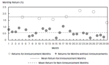
Clearly the returns for announcement months are different from the returns for months without announcement.

The results of the regression are given in Exhibit 29.

	Estimated Coefficients	Standard Error of Coefficients	Calculated Test Statistic
Intercept	0.5629	0.0560	10.0596
EARN	1.2098	0.1158	10.4435

We can draw the following inferences this table:

The t-stats for both the intercept and the slope are high hence we can conclude that both the intercept and the slope are statistically significant.
The intercept is the predicted value of Y when X = 0. Therefore, the intercept (0.5629) is the mean of the returns for non-earnings-announcement months.
The slope coefficient (1.2098) is the difference in means of returns between earnings-announcement and non-announcement months.

5.4 Test of Hypotheses: Level of Significance and p-Values

p-value: At times financial analysts report the p-value or probability value for a particular hypothesis. The p-value is the smallest level of significance at which the null hypothesis can be rejected. It allows the reader to interpret the results rather than be told that a certain hypothesis has been rejected or accepted. In most regression software packages, the p-values printed for regression coefficients apply to a test of the null hypothesis that the true parameter is equal to 0 against the alternative that the parameter is not equal to 0, given the estimated coefficient and the standard error for that coefficient.

Here are a few important points connecting t-statistic and p-value:

Higher the t-statistic, smaller the p-value.
The smaller the p-value, the stronger the evidence to reject the null hypothesis.
Given a p-value, if p-value ≤ α, then reject the null hypothesis H₀. α is the significance level. For example, if we are given a p value of 0.03 or 3%, we can reject the null hypothesis at the 5% significance level, but not at the 1% significance level.

6. Prediction Using Simple Linear Regression and Prediction Intervals

We use regression equations to make predictions about a dependent variable. Let us consider the regression equation: Y = b₀+ b₁X. The predicted value of $\widehat{\ Y}\ =\ \widehat{b_0}+\widehat{b_1}X$ .

The two sources of uncertainty to make a prediction are:

The error term
Uncertainty in predicting the estimated parameters b₀ and b₁

The estimated variance of the prediction error is given by:

$s^2_f=s^2*\left[1+\frac{1}{n}+\frac{{\left(X-\underline{X}\right)}^2}{{\left(n-1\right)s}^2_x}\right]$

Note: You need not memorize this formula, but understand the factors that affect s_f², like higher the n, lower the variance, and the better it is.

The estimated variance depends on:

the squared standard error of estimate, s²
the number of observations, n
the value of the independent variable, X
the estimated mean $\underline{X}$
variance, s², of the independent variable

Once the variance of the prediction error is known, it is easy to determine the confidence interval around the prediction. The steps are:

Make the prediction.
Compute the variance of the prediction error.
Determine t_c at the chosen significance level α.
Compute the (1-α) prediction interval using the formula below: $\hat{Y}\ \pm t_c*s_f$

In our ROA regression model, if a company’s CAPEX is 6%, its forecasted ROA is:

$\widehat{\ Y}\ =\ \widehat{b_0}+\widehat{b_1}X$ = 4.875+1.25 x 6 = 12.375 %

Assuming a 5% significance level (α), two sided, with n − 2 degrees of freedom (so, df = 4), the critical values for the prediction interval are ±2.776.

The standard error of the forecast is:

$s_f=3.49588*\sqrt{\left[1+\frac{1}{6}+\frac{{\left(6-6.1\right)}^2}{122.640}\right]}$ = 3.736912

The 95% prediction interval is:

12.375 ± 2.776 (3.736912)

2.0013 < $\widehat{\ Y}$ < 22.7487

7. Functional Forms for Simple Linear Regression

Economic and financial data often exhibit non-linear relationships. For example, consider a plot of revenues of a company as the dependent variable (Y) and time as the independent variable (X). Such data will often show exponential growth. Using a simple linear model will not fit this data well as illustrated in Exhibit 33 below.

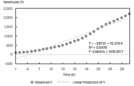
To make the simple linear regression model fit well, we will have to modify either the dependent or the independent variable. The modification process is called ‘transformation’ and the different types of transformations are:

Using the log of the dependent variable
Using the log of the independent variable
Using the square of the independent variable
Differencing the independent variable

In the subsequent sections, we will discuss three commonly used functional forms based on log transformations:

Log-lin model: The dependent variable is logarithmic but the independent variable is linear.
Lin-log model: The dependent variable is linear but the independent variable is logarithmic.
Log-log model: Both the dependent and independent variables are in logarithmic form.

7.1 The Log-Lin Model

In the log-lin model, the dependent variable is logarithmic but the independent variable is linear. The regression equation is expressed as:

ln Y_i = b₀ + b₁X_i

The slope coefficient in this model is the relative change in the dependent variable for an absolute change in the independent variable.

We can transform the Y variable (revenues) in Exhibit 33 into its natural log and then fit the regression line. This is demonstrated in Exhibit 34 below:

We can see that the log-lin model is a better fitting model than the simple linear model for data with exponential growth.

Example: Making forecasts with a log-lin model

Suppose the regression model is: ln Y = −7 + 2X. If X is 2.5% what is the forecasted value of Y?

Solution:

Ln Y = -7 + 2*2.5 = -2

Y = e^-2 = 0.135335

7.2 The Lin-Log Model

In the lin-log model, the dependent variable is linear but the independent variable is logarithmic. The regression equation is expressed as:

Y_i = b₀ + b₁ln X_i

The slope coefficient in this model is the absolute change in the dependent variable for a relative change in the independent variable.

Consider a pot of operating profit margin as the dependent variable (Y) and unit sales as the independent variable (X). The scatter plot and regression line for a sample of 30 companies is shown in Exhibit 35.

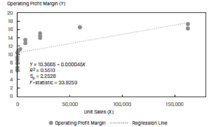
Instead of using the unit sales directly, if we transform the variable and use the natural log of unit sales as the independent variable, we get a much better fit. This is shown in Exhibit 36.

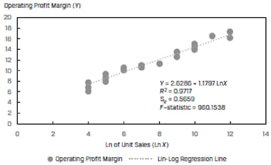
The R² of the model jumps to 97.17% from 55.10%. For this data, the lin-log model has a significantly higher explanatory power as compared to simple linear model.

7.3 The Log-Log Model

In the log-log model, both the dependent and independent variables are in logarithmic form. It is also called the ‘double-log’ model. The regression equation is expressed as:

ln Y_i = b₀ + b₁ln X_i

The slope coefficient in this model is the relative change in the dependent variable for a relative change in the independent variable. The model is often used to calculate elasticities.

Consider a plot of company revenues as the dependent variable (Y) and the advertising spend as a percentage of SG&A, ADVERT, as the independent variable (X). The scatter plot and regression line for a sample company is shown in Exhibit 37 below:

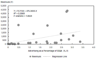
The R² of this model is only 20.89%. If we use the natural logs of both the revenues and ADVERT variables, we get a much better fit. This is shown in Exhibit 38.

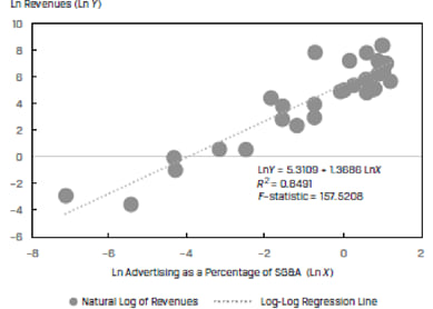
The R² of the model increases by more than 4 times to 84.91% and the F-stat jumps from 7.39 to 157.52. For this data, the log-log model results in a much better fit as compared to the simple linear model.

7.4 Selecting the Correct Functional Form

To select the correct functional form, we can examine the goodness of fit measures:

Coefficient of determination (R²)
F-statistic
Standard error of estimate (SEE)

A model with a high R², high F-stat and low SEE is better.

In addition to these fitness measures, we can also look at the plots of residuals. A good model should show random residuals i.e. the residuals should not be correlated.

Example: Comparing Functional Forms

(This is based on Example 8 of the curriculum.)

An analyst is evaluating the relationship between the annual growth in consumer spending (CONS) in a country and the annual growth in the country’s GDP (GGDP). He estimates the following two models:

	Model 1	Model 2
	GGDP_i = b₀ + b₁CONS_i + ε_i	GGDP_i = b₀ + b₁ln(CONS_i )+ ε_i
Intercept	1.040	1.006
Slope	0.669	1.994
R²	0.788	0.867
SEE	0.404	0.320
F-stat	141.558	247.040