
Statistical inference consists of two branches: 1) hypothesis testing and 2) estimation. Hypothesis testing addresses the question ‘Is the value of this parameter equal to some specific value?’ This is discussed in detail in the next reading. In this section, we will discuss estimation. Estimation seeks to answer the question ‘What is this parameter’s value?’ In estimation, we make the best use of the information in a sample to form one of several types of estimates of the parameter’s value.
A point estimate is a single number that estimates the unknown population parameter.
Interval estimates (or confidence intervals) are a range of values that bracket the unknown population parameter with some specified level of probability.
The formulas that we use to compute the sample mean and all other sample statistics are examples of estimation formulas or estimators. The particular value that we calculate from sample observations using an estimator is called an estimate. For example, the calculated value of the sample mean in a given sample is called a point estimate of the population mean.
The three desirable properties of an estimator are:
A confidence interval is a range of values, within which the actual value of the parameter will lie with a given probability. Confidence interval is calculated as:
Confidence interval = point estimate ± (reliability factor x standard error)
where:
point estimate = a point estimate of the parameter
reliability factor = a number based on the assumed distribution of the point estimate and the degree of confidence (1 – α) for the confidence interval
standard error = standard error of the sample statistic providing the point estimate
The quantity ‘reliability factor x standard error’ is also referred to as the precision of the estimator. Larger values indicate lower precision and vice versa.
Calculating confidence intervals
To calculate a confidence interval for a population mean, refer to the table below and select t statistic or z statistic as per the scenario.
| Sampling from | Small sample size(n<30) | Large sample size(n≥30) | |
| Normal distribution | Variance known | z | z |
| Variance unknown | t | t (or z) | |
| Non –normal distribution | Variance known | NA | z |
| Variance unknown | NA | t (or z) | |
Use the following formulae to calculate the confidence interval:


Sampling from a normal distribution with known variance
The most basic confidence interval for the population mean arises when we are sampling from a normal distribution with known variance.
The confidence interval will be calculated as:
 = sample mean
 = reliability factor
 = standard error
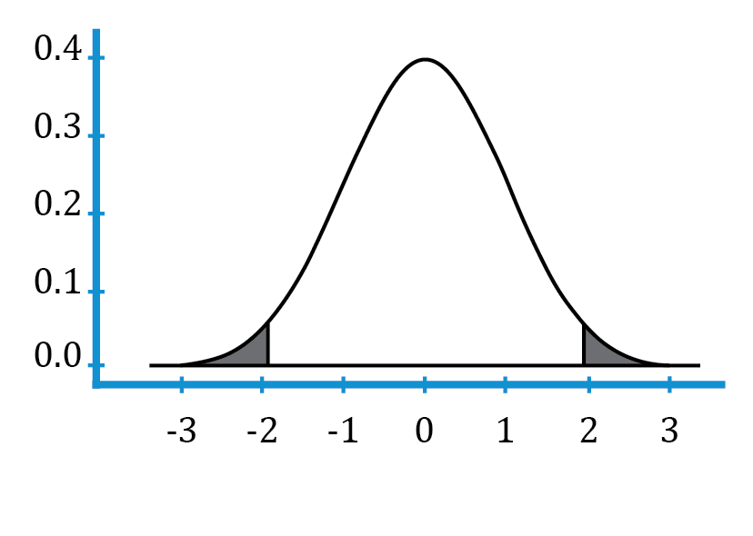
The reliability factor ( ) depends purely on the degree of confidence. If the degree of confidence (1 – α) is 95% or 0.95, the level of significance (α) is 5% or 0.05. α/2 = 0.025. α/2 is the probability in each tail of the standard normal distribution. This is shown in blue in the figure below:
The reliability factors that are most frequently used when we construct confidence intervals based on the standard normal distribution are:
Memorize these confidence intervals and the corresponding reliability factors.
Example
You take a random sample of stocks on the National Stock Exchange (NSE). The sample size is 100 and the average Sharpe ratio is 0.50. Assume that the Sharpe ratios of all stocks on the NSE follow a normal distribution with a standard deviation of 0.30. What is the 90% confidence interval for the mean Sharpe ratio of all stocks on the NSE?
Solution:

Therefore, the 90% confidence interval for the mean Sharpe ratio of all stocks on the NSE is: 0.4505 to 0.5495.
As we increase the degree of confidence, the confidence interval becomes wider. If we use a 95% confidence interval, the reliability factor is 1.96. And the confidence interval ranges from 0.50 – 1.96 x 0.03 to 0.50 + 1.96 x 0.03 which is: 0.4412 to 0.5588. This range is wider than what we had with a 90% confidence interval.
Sampling from a normal distribution with unknown variance
If the distribution of the population is normal with unknown variance, we can use the t-distribution to construct a confidence interval.
The confidence interval can be calculated using the following formula:

This relationship is similar to what we’ve discussed before except here we use the t-distribution. Since the population standard deviation is not known, we have to use the sample standard deviation which is denoted by the symbol ‘s’. We will now see how to read the t-distribution table using an example.
Example
Given a sample size of 20, what is the reliability factor for a 90% confidence level?
Solution:
In order to answer this question, we need to refer to the t-table. A snapshot of the table is given below. This table shows the level of significance for one-tailed probabilities.
| df | P = 0.10 | P = 0.05 | P = 0.025 | P = 0.01 | P = 0.005 |
| 1 | 3.078 | 6.314 | 12.706 | 31.821 | 63.657 |
| 2 | 1.886 | 2.920 | 4.303 | 6.965 | 9.925 |
| 3 | 1.638 | 2.353 | 3.182 | 4.541 | 5.841 |
| 4 | 1.533 | 2.132 | 2.776 | 3.747 | 4.604 |
| 5 | 1.476 | 2.015 | 2.571 | 3.365 | 4.032 |
| 6 | 1.440 | 1.943 | 2.447 | 3.143 | 3.707 |
| 7 | 1.415 | 1.895 | 2.365 | 2.998 | 3.499 |
| 8 | 1.397 | 1.860 | 2.306 | 2.896 | 3.355 |
| 9 | 1.383 | 1.833 | 2.262 | 2.821 | 3.250 |
| 10 | 1.372 | 1.812 | 2.228 | 2.764 | 3.169 |
| 11 | 1.363 | 1.796 | 2.201 | 2.718 | 3.106 |
| 12 | 1.356 | 1.782 | 2.179 | 2.681 | 3.055 |
| 13 | 1.350 | 1.771 | 2.160 | 2.650 | 3.012 |
| 14 | 1.345 | 1.761 | 2.145 | 2.624 | 2.977 |
| 15 | 1.341 | 1.753 | 2.131 | 2.602 | 2.947 |
| 16 | 1.337 | 1.746 | 2.120 | 2.583 | 2.921 |
| 17 | 1.333 | 1.740 | 2.110 | 2.567 | 2.898 |
| 18 | 1.330 | 1.734 | 2.101 | 2.552 | 2.878 |
| 19 | 1.328 | 1.729 | 2.093 | 2.539 | 2.861 |
| 20 | 1.325 | 1.725 | 2.086 | 2.528 | 2.845 |
The degrees of freedom in this case are n – 1 = 20 – 1 = 19. The level of significance is calculated as: 100(1 – α) % = 90% and α = 0.10. In order to calculate the reliability factor ta/2 = t0.10/2 = t0.05 , we look at the row with df = 19. We then look at the column with p = 0.05. The value that satisfies these two criteria is 1.729. This is the reliability factor.
Example
An analyst wants to estimate the return on the Hang Seng Index for the current year using the following data and assumptions:
It is given that the reliability factor for a 95% confidence interval with unknown population variance and sample size greater than 64 is 1.96. Assuming that the index return this year will be the same as it was last year, what is the estimate of the 95% confidence interval for the index’s return this year?
Solution:

Instructor’s Note:
A conservative approach to confidence intervals relies on the t-distribution rather than the normal distribution, and use of the t-distribution will increase the reliability of the confidence interval.
The choice of sample size affects the width of a confidence interval. A larger sample size decreases the width of a confidence interval and improves the precision with which we can estimate the population parameter. This is obvious when we consider the confidence interval relationship, shown below:

All else being equal, when the sample size (n) is increased, the standard error (s/ ) decreases and we have a more precise (narrower) confidence interval. Based on this discussion it might appear that we should use as large a sample size as possible. However, we must consider the following issues:
Resampling is a computational tool in which we repeatedly draw samples from the original observed data sample for the statistical inference of population parameters. Two popular resampling methods are:
Bootstrap
The bootstrap technique is illustrated in the figure below:
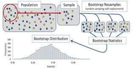
The technique is used when we do not know what the actual population looks like. We simply have a sample of size n drawn from the population. Since the random sample is a good representation of the population, we can simulate sampling from the population by sampling from the observed sample i.e., we treat the randomly drawn sample as if it were the actual population.
Under this technique, samples are constructed by drawing observations from the large sample (of size n) one at a time and returning them to the data sample after they have been chosen. This allows a given observation to be included in a given small sample more than once. This sampling approach is called sampling with replacement.
If we want to calculate the standard error of the sample mean, we take many resamples and calculate the mean of each resample. We then construct a sampling distribution with these resamples. The bootstrap sampling distribution will approximate the true sampling distribution and can be used to estimate the standard error of the sample mean. Similarly, the bootstrap technique can also be used to construct confidence intervals for the statistic or to find other population parameters, such as the median.
Bootstrap is a simple but powerful technique that is particularly useful when no analytical formula is available to estimate the distribution of estimators.
Jackknife
In the Jackknife technique we start with the original observed data sample. Subsequent samples are then created by leaving out one observation at a time from the set (and not replacing it). Thus, for a sample of size n, jackknife usually requires n repetitions. The Jackknife method is frequently used to reduce the bias of an estimator.
Note that bootstrap differs from jackknife in two ways:
There are many issues in sampling. Here we discuss four main issues.
Data-snooping is the practice of analyzing the same data again and again, till a pattern that works is identified.
There are two signs that can warn analysts about the potential existence of data snooping:
The best way to avoid this bias is to test the pattern on out-of-sample data to check if it holds.
When data availability leads to certain assets being excluded from the analysis, the resulting problem is known as sample selection bias.
Two types of sample selection biases are:
A test design is subject to look-ahead bias if it uses information that was not available to market participants at the time the market participants act in the model. For example, an analyst wants to use the company’s book value per share to construct the P/B variable for that particular company. Although the market price of a stock is available for all market participants at the same point in time, fiscal year-end book equity per share might not become publicly available until sometime in the following quarter.
One way to avoid this bias is to use point-in-time (PIT) data. PIT data is stamped with the date when it was released. In the above example, PIT data of P/B would be stamped with the company’s filing or press release date rather than the fiscal quarter end date.
A test design is subject to time-period bias if it is based on a time period that may make the results time-period specific. A short time series is likely to give period-specific results that may not reflect a longer period. If a time series is too long, fundamental structural changes may have occurred in that time period.


Ace the Exam with Active Learning!

Ace the Exam with IFT Notes!

Practice your way to success!

Accelerate your studies!
 Do IFT Mocks to make you exam-ready!


Sign up to get more!