IFT Notes for Level I CFA® Program
LM03 Aggregate Output, Prices and Economic Growth
Part 3
3. Aggregate Demand and Aggregate Supply
Aggregate demand is the quantity of goods and services demanded by consumers (includes households, businesses, government, etc.) at any given price level.
-
- Aggregate supply is the amount of goods and services
- firms will produce in an economy (real GDP) at any given price level.
3.1. Aggregate Demand
The aggregate demand curve (AD) represents the combinations of aggregate income and the price level at which the following two conditions must be satisfied:
- Aggregate expenditure equals aggregate income.
- There must be equilibrium in the money market. e., the available real money supply is willingly held by households and businesses.
The AD curve looks like an ordinary demand curve: quantity demanded increases as price levels decline.
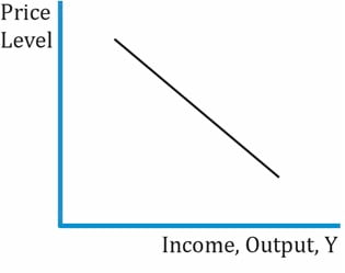
The graph plots price level on the y-axis and aggregate income or real output on the x-axis.
The demand curve in microeconomics and the AD curve here are both negatively sloped. But there are some major differences as listed below:
- The demand curve in microeconomics maps the price of one good to the quantity demanded of that good. Ex: oranges. It is the demand curve for one market. Whereas, the AD curve in macroeconomics represents the average price level in an economy (of all the goods and services demanded) using an indicator such as GDP deflator.
- In microeconomics, we also assume that all other variables such as income and the price of related goods remain constant; and that only the price and quantity demanded of the good change. Whereas in macroeconomics, as we move along the AD curve, income also changes along with the output.
- Aggregate expenditure equals aggregate income.
- There must be equilibrium in the money market. e., the available real money supply is willingly held by households and businesses.
The downward slope of the aggregate demand curve arises as a result of three effects:
- Wealth effect: It is based on the concept of purchasing power of nominal wealth. Nominal wealth does not change, real wealth however fluctuates with the prices of goods and services. An increase in the price level decreases the quantity of goods and services that can be purchased with the fixed quantity of nominal wealth i.e., consumers become less wealthy and will demand fewer goods and services. The opposite is true when price levels decrease.
- Interest rate effect: An increase in price level increases the demand for money – we will need more money to buy the same amount of goods and services. Since the supply of money is fixed, the price of money i.e., interest rate increases. Higher interest rates make borrowing expensive. Businesses make fewer investments when their borrowing costs are high. Consumers also purchase fewer big-ticket items such as automobiles or residential real estate. Thus, the demand for goods and services decreases. The opposite is true when price levels decrease.
- Real exchange rate effect: An increase in price levels increases the real exchange rate (i.e., the domestic currency appreciates). This makes domestic goods more expensive for foreigners, reducing exports. It also makes foreign goods less expensive for the country’s residents, increasing imports. The overall impact is a decrease in demand of domestic goods and services. The opposite is true when price levels decrease.
Why does real exchange rate increase when price levels increase?
When price levels increase, interest rates increase (as discussed above). Foreign investors are attracted by this higher interest rate and they make investments in domestic currency securities. This increases demand for the domestic currency in the foreign exchange market causes it to appreciate. Thus, the real exchange rate increases.
3.2. Aggregate Supply
Aggregate supply curve shows the relationship between domestic output and price level.
The graph below shows the long run, short run, and very short run AS curves (LRAS, SRAS, and VSRAS):
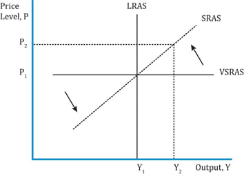
Interpretation of the graph:
- Plots real GDP on the x-axis (remember we had quantity in the microeconomics supply curve).
- Plots price level on the y-axis.
- Very short run: AS curve is almost flat. This is because companies increase or decrease output without changing prices.
- Short run: In the short run, firms consider the price level to decide how much to produce. AS curve is upward sloping – a decrease in the price level reduces the quantity of goods and services supplied. Some costs such as labor and capital are sticky (fixed) in the short run. So, when prices increase, businesses can increase output as it is more attractive (given the high selling prices).
- Long run: In the long run, the AS curve is vertical at a given level of output. We refer to this level of output as ‘potential GDP’ or ‘full-employment GDP’. Aggregate price has no effect on aggregate output because wages, prices and expectations adjust; firms do not decide how much to produce based on the price level. In the long run if prices are up, then costs such as wages also go up and in real terms, nothing has changed.
- In the very long run, there is a shift in the LRAS when costs of production change: labor, capital, natural resources, technological advance, etc. This is discussed in section 4.
There is a distinction in the terms short run and long run as used in micro- and macroeconomics.
- In microeconomics: in the short run, labor is variable, but capital is fixed.
- In macroeconomics: in the short run, wages or some costs are sticky i.e. they do not change. In the long run, all costs change.
Example
What is the relationship between wages and the slope of the SRAS curve?
Solution:
Consider two scenarios: when wages are sticky, and when wages are not sticky.
Wages are sticky: when prices increase, output increases substantially. The slope of SRAS is flatter.
Wages are not sticky: when prices increase, the output does not increase much. The slope of SRAS is steeper.
3.3. Shifts in the Aggregate Demand and Aggregate Supply Curves
The graph below shows LRAS, SRAS and AD curves. This section and the next are based on the interaction of these three curves.
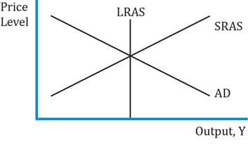
Interpretation of the graph:
- The output level at the intersection of the three curves is called the long run equilibrium level of output or natural level of output.
- The output level is closely related to the level of employment. At the natural level of output, the economy is at the natural rate of unemployment.
- Full employment does not mean 100% employment. It means that there is a natural level of unemployment, which includes people who are in between jobs. The percentage of people who are in between jobs is equal to the percentage of vacancies.
The objective of this section is to understand the interaction of the curves discussed above, what causes a shift in these curves, and to answer these important macroeconomic questions:
- What causes an economy to expand and contract?
- What causes changes in price level and unemployment?
- What determines an economy’s rate of unsustainable growth?
Why are they important? Because GDP growth impacts corporate profits which, in turn, impacts stock prices.
Share on :


 Do IFT Mocks to make you exam-ready!


