LM03 Aggregate Output, Prices and Economic Growth

Part 5

4.  Economic Growth and Sustainability

• Economic growth is measured as the annual percentage change in real GDP or the annual change in real per capita GDP. Growth in real GDP measures how the quantity of goods and services produced has increased from one year to the next.
• Per capita GDP is the . It is a good measure as it tells us whether the standard of living is improving or not. For instance, if the GDP grew by 3% in a year and the population also grew by 3%, then there is no improvement in the standard of living. But, if GDP grows at a higher rate than the population, then the per capita GDP would increase and so would the potential standard of living.
• Sustainable rate of economic growth is the rate of increase in the economy’s productive capacity or potential GDP. Any growth should be sustainable over the long term. A sudden, rapid increase in GDP is difficult to sustain as it leads to inflation, environmental damage etc.

What is the difference between saying that there is a 4% change in real GDP and saying that there is a 4% change in potential GDP? As an investor, what will excite you more?

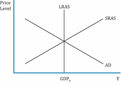
This is an economy in long-run equilibrium as the intersection of aggregate demand (AD) and short-run aggregate supply (SRAS) lies on the long-run aggregate supply curve (LRAS). Point GDP_P on the x-axis represents the potential GDP or productive capacity. The LRAS is shifting to the right, and the overall productive capacity of the economy is going up.

In contrast, if the real GDP increases by 4%, then it means the AD has increased, and the AD curve shifts up to the right. The corresponding GDP now is GDP_real. The equilibrium point has gone up in the short-term and it is likely it will come back to a point on the LRAS. As an investor, we will be happy if the LRAS moves to the right as it means an increase in productive capacity.

4.1. The Production Function and Potential GDP

The Solow growth model is the starting point for analyzing the drivers of long-term growth in any economy. With this model, one can analyze why the growth in one country differs from another. This model is relevant in determining the factors that cause the LRAS curve to shift permanently to the right (increase in productive capacity of an economy).

According to the neo-classical model (also called the Solow growth model), productive capacity (potential GDP) increases for the following reasons:

1. Accumulation of factors of production such as capital, labor, and raw materials.
2. Discovery of new technologies that give production efficiency.

The Solow model builds on the Cobb-Douglas production function, which we have seen earlier in microeconomics, and adds capital accumulation to it. It is based on the assumption that capital accumulation in the long run fuels economic growth. The Solow model is based on a production function such as: Y = A * F (L, K) which means the output is a function of labor and capital, and total factor productivity.

The Solow model uses four variables:

• Y is the level of aggregate output in the economy.
• A represents total factor productivity and is a measure of efficiency.
• L is the quantity of labor or the number of workers in the economy.
• K is the capital stock.

Recall that the production function is based on two assumptions:

• Constant returns to scale for two variables (capital and labor): If capital and labor inputs are increased by x percentage, then output also increases by x So, if all inputs are doubled, then the output doubles as well.
• Diminishing marginal productivity: At some point, the output from each additional input will decline. Consider a simple economy whose output is primarily agricultural products, and assume traditional methods, such as bullock carts, are used for farming.
  • If bullock carts are replaced with tractors, then the increase in capital causes output to increase rapidly.
  • With more capital per farmer, the economy produces more output per farmer.
  • But at some point, each additional unit of capital increases the output per farmer by less than the previous unit of capital; the increase in output is only marginal. This is diminishing marginal productivity.

Diminishing marginal productivity has two major implications on potential GDP:

1. Long-term sustainable growth cannot rely solely on capital deepening investment. Capital deepening is increasing the amount of capital per worker (labor). We just saw in the farming example, that increasing capital stock relative to labor will lead to diminishing returns. So, it is not sustainable to grow an economy by adding more and more capital in the long run.
2. But, adding more capital in developing countries leads to a substantially higher productivity (a higher rate of output) relative to developed countries. It implies that the growth rate of developing countries must exceed that of developed countries. Ex: think of investing USD 1 million on new farming techniques in India and the US in 2000. The spurt in output in India must have been much higher than that in the US. This also means that there should be a convergence of incomes between developed and developing countries over time.

Growth Accounting Equation

The following equation is the model developed by Solow to show the relationship between growth in potential output and growth in technology, capital, and labor.
Growth in potential GDP = growth in technology + W_L(growth in labor) + W_C(growth in capital)
W_L and W_C are the relative share of labor and capital in the national income
Growth in per capita potential GDP = growth in technology + W_C (growth in K/L ratio)
Example: In a given economy, the growth in potential GDP is given by:
2.0 + 0.7 (growth in labor) + 0.3 (growth in capital)
How should we interpret 2, 0.7 and 0.3?

Interpretation:
2.0: growth in technology.
0.7: relative share of labor in national income.
0.3: relative share of capital in national income.

In other words, if all else stays constant, a 1% growth in labor will result in 0.7% growth in potential GDP. Or, if all else stays constant, a 1% growth in capital will result in 0.3% growth in potential GDP.

4.2. Sources of Economic Growth

Increase in Labor Supply

Increase in labor supply leads to an increase in economic growth. Labor force is the number of people available for work from the working age population. This includes unemployed people who are looking for work.

Total hours worked = Labor force * average hours worked per worker

Increase in Human Capital

This is the quality of the workforce i.e. the skill and knowledge of the workers. Investment in education and on-the-job training improves human capital, which in turn causes the production function to shift upward, and improves productivity/standard of living/economic growth. The spillover effect is the effect of this investment in human capital on the people around.

Increase in Physical Capital

This refers to buildings, machinery, and equipment. If net investment is positive, then physical capital is growing. Countries with a higher rate of net investment have a higher GDP growth. Ex: China, India, and South Korea.

Investments in Technology

Spending on R&D leads to discoveries or technological improvements that make it possible to increase a firm’s output with the same inputs. Ex: growth in IT; semiconductor industries. This is one factor that allows an economy to grow because other inputs (capital, labor) face diminishing marginal returns. The faster the growth in technological change, the greater the growth in productivity and GDP. TFP represents the amount by which an output increases due to improvements in the production process.

TFP Growth = Growth in potential GDP – [W_L(Growth in labor) + W_C(Growth in capital)]

Technology is the main factor that affects economic growth in developed countries.

Natural Resources: comprises renewable (can be replenished, such as trees and water) and non-renewable resources (coal and oil). Higher natural resources lead to higher growth.

Public infrastructure: Examples of public infrastructure include: roads, water systems, mass transportation, airports, utilities etc. These investments create externalities which boost the production of private goods and services. The benefits derived from public infrastructure investments extend beyond the direct costs incurred in creating them.

Other factors driving growth: Other factors such as R&D and public education also produce positive externalities that can boost economic growth.

However, some factors such as pollution can produce negative externalities and limit economic growth. For example, carbon dioxide emissions usually rise with economic growth, the resultant climate change impose a cost on the global economy in terms of economic activity, food production, health and habitability.

Improvements in a country’s legal and political environment can also improve economic growth.

4.3. Measures of Sustainable Growth

• It is not easy to measure sustainable GDP as it depends on growth of technological change, capital, labor and natural resources. This is because there is no observed data on TFP or potential GDP and hence it must be estimated.
• Labor productivity is easier to measure. It is the amount of output produced by an average worker in one hour.
  Labor productivity =
  
• An increase in any of the factors – capital, technology – improves productivity of the labor force.
• Level of labor productivity: Higher labor productivity means more goods and services per person. This, in turn, depends on the level of human and physical stock. The higher the accumulated capital, the higher the productivity.
• Growth rate of labor productivity: % increase in productivity over a year.
• Labor productivity can be used to estimate the rate of sustainable growth of the economy and differences in living standards.

Potential GDP can be expressed as:

Potential GDP = Aggregate hours worked * Labor productivity.

Converting the above equation in terms of growth rates we get:

Potential growth rate = long-term growth rate of labor force + long-term labor productivity growth rate.

Share on :