LM01 Topics in Demand and Supply Analysis

Part 1

1.  Introduction

Economics is a discipline that deals with factors affecting the production, distribution, and consumption of goods and services. It is divided into two broad areas: microeconomics and macroeconomics.

Macroeconomics deals with the production and consumption of the overall economy. It focuses on aggregate economic quantities such as gross domestic product, gross national income, and national output.

Microeconomics deals with demand and supply of goods and services at a micro level, such as individual consumers and businesses. According to microeconomics, private economic units can be divided into two groups of study:

• The theory of the consumer that focuses on the consumption of goods and services.
• The theory of the firm that focuses on the supply of goods and services.

This reading focuses on microeconomics and covers the demand and supply side of the market.

2.  Demand Concepts

Demand is the willingness and ability of consumers to purchase a given amount of good or service at a given price. The law of demand states that as the price of a good rises, consumers will want to buy less of it. Similarly, as price falls, the quantity demanded increases. Apart from the good’s own price, other factors that impact consumer demand include prices of other substitute and complement goods, customers’ incomes, and individual tastes and preferences.

The general form of a demand function is shown below:

Demand function for good A: Q^D = f(P_A, I, P_B … … )

where:

Q^D = quantity demanded of some good.

I = consumer’s income.

P_A = price per unit of a related good A.

P_B = price per unit of a related good B.

Let us take a hypothetical example of a demand function for the quantity of chairs demanded in a small town. The demand function is given by:

Q_D = 10 – 0.5P + 0.06I – 0.01P_T

In the equation above, I is the consumers’ income and P_T is the price of tables. Note the signs of the coefficients for income and price of tables. Chairs and tables are complementary products as they sell together. The quantity demanded for chairs, Q_D, and price of tables, P_T, are inversely related. If the price of a table increases, then the quantity demanded for chairs decreases. Similarly, income has a positive coefficient. If income increases, then the quantity demanded for chairs increases.

Now, let us assume that the consumers’ income and the price of the table are fixed at a particular point in time. If the values of I and P_T are 1633.33 and 800.00 respectively, then the quantity demanded can be rewritten as:

Q^D = 100 – 0.5P

The inverse demand function expresses the simple demand function in terms of price. The above function can be rearranged and expressed in terms of P as:

P = 200 – 2Q

A demand curve is a graphical representation of the inverse demand function. The demand curve plots the price on the y-axis and the quantity on the x-axis.  It shows the quantity of a good that consumers are willing to buy at any given price, all else equal.

Let us plot the demand curve given by the equation P = 200 – 2Q. Here, the intercept is 200 and the slope of the curve is -2. The slope of the demand curve is measured as the change in price divided by the change in quantity.

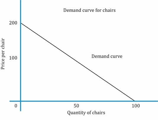
Interpretation of the graph:

• The demand curve shows the highest quantity consumers are willing to purchase at each price. When P = 200, the highest quantity consumers are willing to purchase is 0.
• Similarly, the demand curve also shows the highest price consumers are willing to pay for each quantity. When Q = 50, the highest price consumers are willing to pay is 100.
• The slope of the demand curve is negative. This implies that as price decreases, the quantity demanded increases.
• Movement along the demand curve: When a good’s own price changes, the quantity demanded changes, all else equal. This change is called a movement along the demand curve. For instance, as price increases from 100 to 110, quantity decreases along the line (demand curve) from 50 to 45.
• Shift in the demand curve: A change in the value of any other variable will cause the demand curve to shift. This is called change in demand. For instance, shift in demand is caused by changes in consumers’ incomes, price of substitutes, and price of complements.

3.     Own Price Elasticity of Demand

Own-price elasticity of demand can be expressed as the percentage change in quantity divided by the percentage change in price.

Before we go further, let us refresh a basic mathematical principle. Consider a simple equation:

A = 10 + 5B – 6C + 8D. Given this equation,  is equal to the coefficient of B which is 5. Similarly,  is equal to the coefficient of C which is -6.

Going back to our demand function, Q^D = 100 – 0.5P. Based on the mathematical principle we just discussed, = -0.5. Assume the price is $60; the quantity demanded at this price will be 70. The own-price elasticity of demand is: -0.5 x 60/70 = -0.4. This implies that when the price is $60, a 1% increase in price results in a 0.4% decrease in the quantity demanded for chairs.

Instructor’s Note

Own-price elasticity of demand is usually negative.

Elastic, Inelastic, and Unit Elastic

For all linear demand curves, elasticity varies depending on where it is calculated. Let us go back to the own-price elasticity of demand for chairs to see which parts of the demand curve are inelastic, elastic and unit elastic.

• Inelastic: When elasticity is less than one, demand is inelastic. At low prices, quantity demanded is high. This causes the P/Q ratio to be small which results in low elasticity.
• Unit elastic: An elasticity of 1 is said to be unit elastic.
• Elastic: When elasticity is greater than one, demand is elastic. At high prices, quantity demanded is low. This causes the P/Q ratio to be high which results in high elasticity.

These scenarios are shown in the figure below:

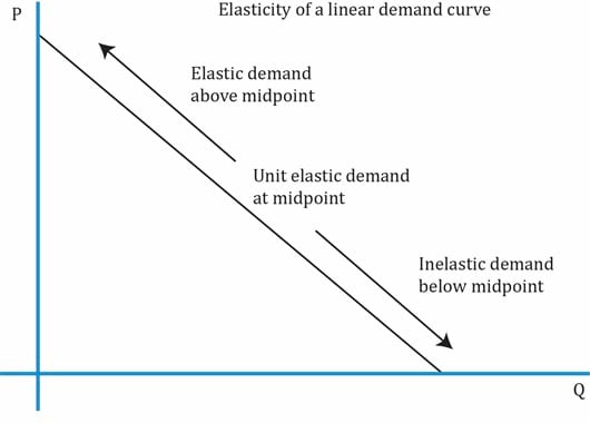
Inference:

• The top part of the demand curve is elastic.
• Somewhere in the middle, it is unit elastic.
• The bottom part of the demand curve is inelastic.
• If the demand curve is steeper, it will be relatively more inelastic.
• If the demand curve is flatter, it will be relatively more elastic.

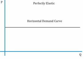
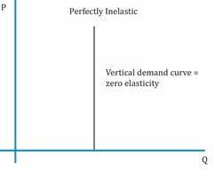
Extremes of Price Elasticity

There are two special cases of linear demand curves in which the elasticity is the same at all points – perfectly elastic and perfectly inelastic – though it is difficult to find real life examples. Demand is perfectly inelastic (represented by a vertical demand curve) when the quantity demanded is the same over a price range. Demand is perfectly elastic for a given price (represented by a horizontal demand curve) when a change in price will cause the quantity demanded to reduce to zero.

Elasticity
Perfectly Elastic	Perfectly Inelastic
Horizontal demand curve	Vertical demand curve.
Elasticity = ∞	Elasticity = 0
A small change in price can lead to infinitely large change in quantity. All producers must sell at the market price, or else consumers will shift to substitutes. Example: Gourmet food items.	A change in price has no change in quantity demanded. Example: generic food such as bread.

4. Predicting Demand Elasticity, Price Elasticity and Total Expenditure

Factors that affect Demand Elasticity

The factors that help in determining whether the demand for a product is highly elastic are as follows:

• Substitutes: If there are close substitutes for a good and the price of the good increases, then the quantity demanded for the good will decrease substantially implying the demand is highly elastic. If there are no close substitutes, the demand is less elastic.
• Portion of budget spent on a good: If people spend a large part of their income on a good, then the demand is likely to be elastic, e.g. cars. On the other hand, if people spend only a small portion of their income on a good, then the demand is likely to be inelastic, e.g. chocolates.
• Time horizon: Long-run demand is more elastic than the short-run demand for most products as people take time to adjust their consumption (quantity demanded) to the new prices. In the long run, consumers will find alternatives. For instance, if prices of cars increase, consumers will find alternative modes of transport in the long run.
• Discretionary vs. nondiscretionary: The demand for necessary goods is less elastic, e.g. bread. While the demand for discretionary goods is more elastic, e.g. vacations.

Elasticity and Total Expenditure

Total expenditure is the total amount consumers spend on a product. It is the price multiplied by the quantity.

Total expenditure = P x Q = Price per unit x quantity or number of units sold

Elastic demand: When demand is elastic, a 1% decrease in price causes a quantity demanded to increase by more than 1%. As a result, total expenditure increases.

Inelastic demand: When demand is inelastic, a 1% decrease in price causes quantity demanded to increase by less than 1%. As a result, total expenditure decreases.

Unit elastic: Total expenditure does not change at the point where demand is unit elastic.

The relationship between change in price and total expenditure is summarized in the table below:

Elasticity and Expenditure
Own-price elasticity of demand = Total expenditure = P x Q = Price per unit x quantity or number of units sold
Ed > 1: elastic demand	Price and total expenditure move in opposite directions
Ed = 1: unitary elastic	Change in price has no effect on total expenditure
Ed < 1: inelastic demand	Price and total expenditure move in the same direction

Share on :