
Shifts in Aggregate Demand
In this section, we look at the factors that cause an aggregate demand curve to shift.
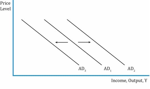
| Shift in the Aggregate Demand Curve | ||
| To determine shift in AD, use the equation C + I + G + (X – M) | ||
| An Increase in the following factors | Shifts in the AD Curve | Reason |
| Stock prices | Right | Higher consumption. This is also called the wealth effect. Increase in stock prices à increase in household wealth à need to save decreases as future goals are met à more income spent on consumption à shift in the demand curve. |
| Housing prices | Right | Higher consumption. Wealth effect. |
| Consumer confidence | Right | Consumers confident about future & job security à spend more of their disposable income. |
| Business confidence | Right | Companies optimistic about future growth prospects à increase in investments. |
| Capacity utilization | Right | Increase in investment spending if companies are operating at near or full capacity. |
| Government spending | Right | Increase in government spending (fiscal policy). |
| Taxes | Left | Higher taxes à lower disposable income à lower consumption. Lower investment spending by businesses. |
| Bank reserves | Right | More money supply. Interest rates are low. Investment is higher. Higher income and higher expenditure. Consumers hold real money balances. |
| Exchange rate | Left | Domestic currency is stronger. Lower exports. Higher imports. Net exports are lower. |
| Global growth | Right | Faster economic growth in foreign markets à foreign consumers buy domestic products à exports are higher. Net exports are higher. |
Note: Government spending and taxes are part of fiscal policy. Bank reserves and the exchange rate are part of monetary policy. These are covered in the next two readings.
A few other points related to AD curve:
Shifts in Aggregate Supply
In the AS curve, the price level is on the y-axis and output on the x-axis. The LRAS is a vertical line while the SRAS is a positively sloped curve. The factors in bold in the first column affect both the SRAS and the LRAS curve to shift, while the remaining factors affect only the SRAS curve.
| Shift in the Aggregate Supply Curve | |||
| An Increase in the following factors | Shifts SRAS | Shifts LRAS | Reason |
| Supply of labor | Right | Right | Increases resource base. Labor supply depends on the labor participation rate, growth of population, etc. |
| Supply of natural resources | Right | Right | Increases resource base. |
| Supply of human capital | Right | Right | Increases resource base. Improvement in quality of labor. |
| Supply of physical capital | Right | Right | More efficiency with better equipment à more output. |
| Productivity and technology | Right | Right | Higher productivity à higher efficiency and amount of output produced by workers in a given time. Decreases labor cost; higher profitability. |
| Nominal wages | Left | No impact | Largest component of a company’s costs are wages. Higher wages à higher labor cost. |
| Input prices | Left | No impact | Increases cost of production. |
| Expectation of future prices | Right | No impact | Anticipating higher future prices à higher profitability. |
| Business taxes | Left | No impact | Increases cost of production. |
| Subsidy | Right | No impact | Lowers cost of production. |
| Exchange rate | Right | No impact | Lowers cost of production.
Many countries import raw materials. Ex: Japan. If the domestic currency is stronger, then imports are cheaper. |
The position of the LRAS curve is determined by the potential output of the economy. Potential GDP measures the productive capacity of the economy and is the level of real GDP that can be produced at full employment.
Short-run macroeconomic equilibrium may occur at a level above or below full employment; there are four possible types of macroeconomic equilibrium:
The price level and output at the point where AD and SRAS curves intersect is called the short-run macroeconomic equilibrium. At this point, the aggregate quantity demanded = aggregate quantity supplied. Let us denote the real GDP at equilibrium as Y1. If we are to the left of this point, then the level of unemployment is higher than the natural level of employment.
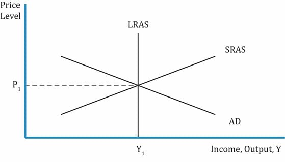
Long-run macroeconomic equilibrium:
The graph below shows a long-run macroeconomic equilibrium.
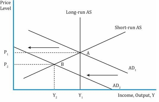
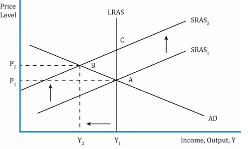
Recessionary gap:
The graph below shows a recessionary gap.
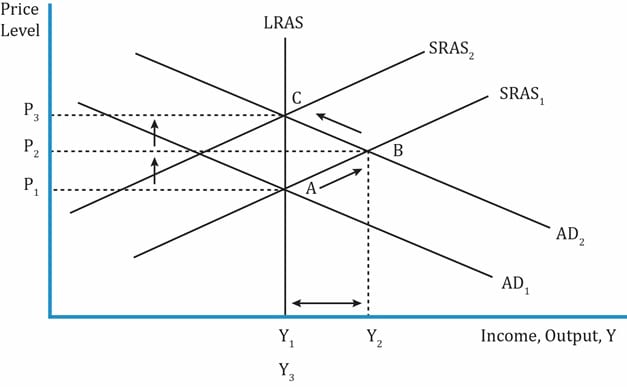
Inflationary gap:
The graph below shows an inflationary gap.
Stagflation:
The graph below shows a stagflation scenario.
Example
The table below shows the effect of changes in AS and AD on real GDP. Fill the last two columns in the table below for different combinations of AD and AS in the first two columns.
| Effect of changes in AD and/or AS | |||
| Change in AS | Change in AD | Effect on Real GDP | Effect on Aggregate Price Level |
| Increase | |||
| Decrease | |||
| Increase | |||
| Decrease | |||
| Increase | Increase | ||
| Decrease | Decrease | ||
| Increase | Decrease | ||
| Decrease | Increase | ||
Solution:
| Change in AS | Change in AD | Effect on Real GDP | Effect on Aggregate Price Level |
| Increase | Increase. Lowers unemployment. | Increase | |
| Decrease | Decrease. Increases unemployment. | Decrease | |
| Increase | Increase. Lowers unemployment. | Decrease | |
| Decrease | Decrease. Increases unemployment. | Increase | |
| Increase | Increase | Increase | Indeterminate |
| Decrease | Decrease | Decrease | Indeterminate |
| Increase | Decrease | Indeterminate | Decrease |
| Decrease | Increase | Indeterminate | Increase |


Ace the Exam with IFT Notes!

Ace the Exam with Active Learning!

Practice your way to success!
 Do IFT Mocks to make you exam-ready!

Accelerate your studies!


Sign up to get more!