LM02 The Firm and Market Structures

Part 4

14. Monopoly & Demand & Supply & Optimal Price and Output in Monopoly Markets

This is a market structure in which a single company makes up the entire market. It is on the opposite end of the spectrum as compared to perfect competition.

Characteristics:

• Single seller of a highly differentiated product.
• No close substitute.
• Significant barriers to entry.
• Considerable pricing power.
• Product is differentiated through non-price strategies such as advertising.

Ex: Government created monopolies such as electricity or water supply in a major city.

How monopolies are created:

• Patent or copyright.
• Control over critical resources – Ex: De Beers’ control of mining resources in South Africa.
• Government authorization – Ex: utilities like electricity, water, etc.
• Strong brand loyalty which creates high barriers to entry (Rolex watches).
• Network effect (Microsoft).

A natural monopoly is one where cost decreases with quantity. The firm is able to meet most of the quantity demanded at a low cost, making it difficult for new firms to enter the market.

14.1. Demand Analysis in Monopoly Markets

The demand curve in a monopoly is downward sloping. Let us take the example of electricity. As a consumer, the quantity demanded is still dependent on the price. To sell an additional unit of the good, the producer must lower the price to increase quantity. This explains why the demand curve is downward sloping.

Let us say the quantity demanded is given by:

Q = 400 – 0.5P

Rewriting the demand function, we get P = 800 – 2Q

TR = P * Q = 800Q – 2Q²

MR =  = 800 – 4Q

AR = 800 – 2Q

The average revenue for a demand curve is the same as the demand curve.

14.2. Supply Analysis in Monopoly Markets

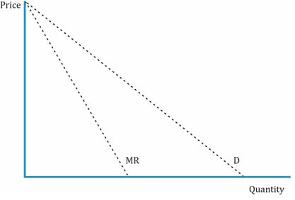
The graph below shows the demand, MR, AC, and MC curves for a monopoly firm.

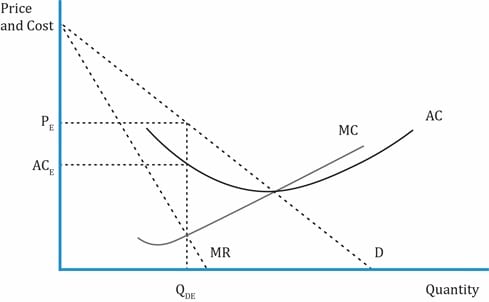
The profit maximizing level of output, Q_, is when MR = MC. The corresponding price, P_E, at this level of output is determined by the demand curve.

Profit is based on the demand curve = TR – TC. Let’s say TC is given by:

TC = 20000 + 50Q + 3Q² (the TC equation will be given; you need not derive it)

From TC, we can derive MC = = 50 + 6Q.

Given the total cost function, you can derive the MC curve as shown above. Supply and demand can be equated to determine the profit-maximizing output.

800 – 4Q = 50 + 6Q

Q = = 75

14.3. Optimal Price and Output in Monopoly Markets

In the previous section, we calculated the optimal output by equating MR = MC.

Another way of determining the profit-maximizing output is to equate = 0. At this point there is no change in profit when output changes.

The price at the profit-maximizing output level of 75 is:

P = 800 – 2 (75) = 650

If π = -20000 + 750Q – 5Q², at what quantity is profit maximized?

= 750 – 10 Q.

Equating it to 0, we get 750 – 10Q = 0 → Q = 75.

Relationship between MR and price elasticity is: MR = P [1- ]

Profit maximization condition in monopoly: MR = MC

MC = P [1- ]

Profit-maximizing price =

If MC = 75 and the own price elasticity of demand = 1.5, what is the profit-maximizing price?

Profit-maximizing price = = 225.

Natural Monopoly in Regulated Pricing Environment

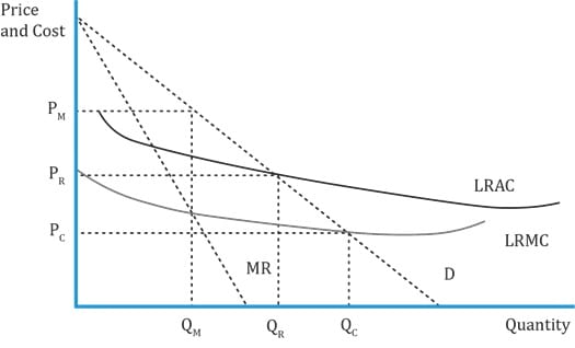
A natural monopoly is a market where the average cost of production falls over the relevant range of consumer demand. There are three possible cases for output and pricing:

• Left unregulated, monopoly will maximize profits by producing the quantity for which MR = MC
• Government regulation may attempt to improve resource allocation by requiring average cost pricing or marginal cost pricing.

15. Price Discrimination and Consumer Surplus

What a monopolist charges for their product and how much quantity is supplied lie on two extremes: on one end the price and quantity supplied may be equal to that of perfect competition where there is a uniform price, and on the other end is discriminating consumers on some grounds, which leads to different prices for the same product.

Ex: In restaurants, lunch is cheaper than dinner, or weekday prices are different than Friday-Sunday prices.

First degree price discrimination:

• Consumer is charged maximum he is willing to pay; sellers are able to capture all consumer surplus.
• Consumers are charged different prices for the same product (airline tickets).
• The monopolist is able to measure exactly how much each consumer is willing to pay and what their preferences are. Prices vary for each consumer and unit. In some cases, public price disclosure may not be permitted. So, one customer is not aware of how much another customer is paying for the same product.

Second degree price discrimination:

• Unlike first degree, the monopolist is not able to exactly measure consumer’s preferences, or his willingness to pay before pricing the product.
• Consumer charged differently based on how much he values the product. Ex: a TI BAII Plus Professional.
• Another instance is where consumers are charged differently based on the quantity sold. Ex: Quantity discounts (the price per unit decreases as the number of units sold to a consumer are higher) are often seen. Family fare airline tickets (different fare if the number of passengers traveling is more than 2) is another example.
• Some amount of consumer surplus is captured in this form of discrimination.

Third degree price discrimination:

• Consumers segregated based on demographic or other traits (gender, age).
• Example: One-day (business travelers) vs. round-trip airline tickets, milk prices within the state/outside state. Student vs. professional version of many software packages.

Example

My monthly demand for visits to the local gym is given by: Q = 25 – 5P where Q is the number of visits per month and P is the price per visit. The gym’s marginal cost is 1 per visit.

1. What the X-axis and Y-axis intercepts for the demand curve?
2. If the gym charged a price per visit equal to its marginal cost, how many visits would I make per month?
3. What is my surplus at this price?
4. How much could the club charge per month for a membership fee?

Solution:

1. Q = 25 – 5P, P = 5 –

X-axis intercept when P = 0 is Q = 25.

Y-axis intercept when Q = 0 is P = 5.

2. If P = 1, then Q = 25 – 5 * 1 = 20

I would make 20 visits per month.

3. Consumer surplus =
4. The club could charge a membership fee of 40 to extract all the consumer surplus. In addition, it must charge 1 per visit. This pricing method is called a two-part tariff.

Example

Monopolists have considerable pricing power and may charge consumers in different ways. Exporters charging higher prices for denim jeans in the international market compared to local markets is an example of:

1. First-degree price discrimination.
2. Second-degree price discrimination.
3. Third-degree price discrimination.

Solution: C

Third-degree price discrimination occurs when customers are segregated by demographics. Dividing the customers into two groups, local and international; and charging two different prices is an example of third-degree price discrimination. The first degree of price discrimination allows a monopolist to charge the highest price each customer is willing to pay. The second degree of price discrimination is when the monopolist charges different people different prices using the quantity purchased as an indicator of how highly the customer values the product.

16. Factors Affecting Long-Run Equilibrium in Monopoly Markets

Unregulated monopolies can earn economic profits in the long run as all factors of production are variable in the long run.

For regulated monopolies, there are several possible solutions in the long run:

• Price = marginal cost. But this will be less than long-run average cost. So there must be a government subsidy to compensate for the loss. Ex: Amtrak.
• National ownership. But the problem is consumers are not willing to accept price increases once the price is fixed even if the input price increases.
• Regulated, authorized monopoly. P = LRAC. Investors make a normal profit, but the challenge is to identify the monopolist’s realistic LRAC.
• Franchise monopolistic firm through a bidding war to select a firm whose P = LRAC.

Share on :