IFT Notes for Level I CFA® Program
LM02 The Firm and Market Structures
Part 2
6. Supply Analysis & Optimal Price and Optimal Output in Perfectly Competitive Markets
When market prices increase, firms supply greater quantities. The market supply curve is the sum of the supply curves of the individual firms. Some key terms (covered earlier) are:
- Economic costs: These include all explicit costs and implicit opportunity costs that are required to acquire a resource or keep it in production.
- Opportunity cost: This is the value of the next best opportunity that is foregone when another alternative is chosen. For example, if a stay-at-home mom was employed, she would earn $90,000 a year. In this case, the mother staying home had given up the opportunity to work, and with it an income of $90,000.
- Economic profit = total revenue minus opportunity cost.
3.3. Optimal Price and Output in Perfectly Competitive Markets
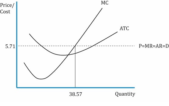
To determine the equilibrium price and quantity, we must equate market supply and demand functions. Say for a given industry the demand function is: P = 25 – 0.5QD and the supply function is P = -2 + 0.2QS. We would solve for the equilibrium quantity and price by using the equation: P = 25 – 0.5QD = -2 + 0.2QS. Solving for Q, we get 38.57. Similarly, P = 5.71.
The equilibrium (optimal) price and quantity are 5.71 and 38.57 respectively. Each firm is a price taker, which means each firm in the market must sell the product at 5.71. The equilibrium price is determined by the market and each firm is too small to influence the price. If a firm decides to sell the product at 6 instead of 5.71, then it will not find any consumers who are willing to buy at that price. The quantity produced by each firm is not determined by the market. A firm may produce 10 or 10,000 units of the product to sell at 5.71 each. The optimal quantity is determined by the firm’s cost curves.
The graph below plots MC and ATC curves for an individual firm in a perfectly competitive market selling oranges at the market price of 5.71.
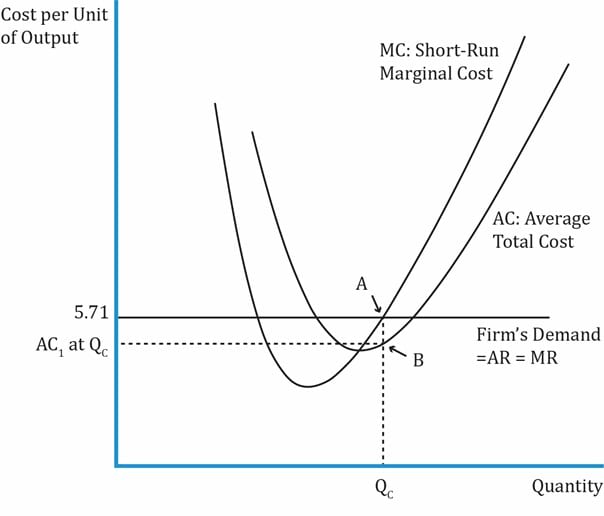
Interpretation of the graph:
- This graph plots cost per unit on the y-axis and output quantity on the x-axis.
- Generally, cost curves are U-shaped because of the law of diminishing returns. The cost of selling oranges comes down as the quantity increases until it reaches a minimum. Beyond that point (optimal quantity), increasing the output quantity increases the cost.
- MC curve intersects the ATC curve at its minimum point.
- The horizontal line shows the market price of 5.71. It is also the marginal revenue, average revenue and the demand curve (perfectly elastic). P = MR = AR = D.
- Profit-maximization condition: The firm’s profit-maximizing condition is MR = MC. The corresponding quantity is QC.
- Link between a firm’s supply and MC curve: A firm’s supply curve is the portion of the firm’s MC curve above the minimum point of its AVC curve. This is the upward-sloping portion of the MC curve.
- Assume the market price of oranges comes down to 4, the total fixed cost is 0, and the variable cost of producing each orange is 5; ATC is 5. So, will the firm sell oranges? No, as the cost is more than the market price. The supply will be zero. That explains why the firm’s supply curve is an MC curve above the minimum point of ATC.
- Economic profit = TR – TC.
3.4. Factors Affecting Long-Run Equilibrium in Perfectly Competitive Markets
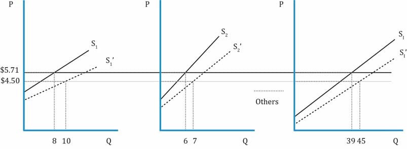
- Let us continue our orange example. Other firms will be attracted to enter the market to sell oranges when they see this firm makes a positive economic profit. This means more output (supply of oranges), which shifts the supply curve to the right.
- For a given demand curve, the supply curve shifts to the right. Because of the increase in output quantity, the price comes down.
- In the long run, the firm will operate at a point where equilibrium price = MC = MR = minimum ATC. Economic profit will be zero because TR = TC. As economic profit is zero, no more firms will enter the perfectly competitive market.
8. Supply, Demand, Optimal Pricing, and Optimal Output under Monopolistic Competition
This is a market where there are many sellers of slightly differentiated products. Product differentiation is the key here. Ex: Burgers sold by KFC, McDonalds, Burger King, etc.
If the firm is able to successfully differentiate the product (e.g. Harley Davidson motorcycles), then the firm acts like a small monopoly.
Characteristics:
- There are a large number of potential buyers and sellers.
- The products offered by each seller are close substitutes for the products offered by other firms, and each firm tries to make its product look different.
- Entry into and exit from the market is possible at fairly low costs.
- Firms have some pricing power.
- Firms differentiate their products through advertising and other non-price strategies.
8.1. Demand Analysis in Monopolistically Competitive Markets
The graph below shows the marginal cost (MC), demand and marginal revenue (MR) curve for a monopolistic firm.
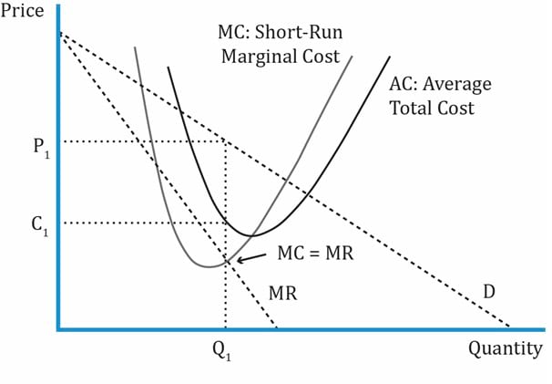
- Since the products are unique, a monopolistic firm has a downward sloping demand curve. MR is steeper and lies below the demand curve.
- Let us consider the toothpaste market. If consumers believe using Sensodyne toothpaste will relieve them of toothaches, then they will buy the product. However, the firm will have a downward sloping curve because if the prices are very high, then consumers will not buy the product, and will look for alternatives. Conversely, demand increases when the price decreases.
- Price and quantity demanded are inversely related.
- In the short run, the profit-maximizing quantity is MR = MC. This is Q1 in the graph. The price is then determined based on the demand curve. This is P1 in the graph.
- Because the product is differentiated, firms have some pricing power and charge what is determined by the demand curve. But each time a new firm enters the market, the demand curves of other firms fall (i.e., they lose a part of the market share). Since there is high competition, the products are often priced closed to each other.
- Demand is elastic at higher prices and inelastic at lower prices.
- Total revenue = P1 * Q1
- Cost = C1 * Q1
- In the short run, economic profit = (P1 * Q1) – (C1 * Q1)
8.2. Supply Analysis in Monopolistically Competitive Markets
8.3 Optimal Price and Output in Monopolistically Competitive Markets
Key points related to supply analysis in the context of monopolistic completion are:
- Output is based on MR = MC.
- Price is determined based on the demand curve.
- The supply function is not well-defined in monopolistic competition.
- Recall that in perfect competition, a firm’s output does not affect the price as all units sell at the same price (horizontal demand curve). They are price takers. P = MR = MC. But, how much a firm produced was dependent on its MC curve. In the short run, the firm’s supply curve was the MC curve above the minimum point of the AVC curve. The MR curve was a flat line and the same as the market price at that point.
- But, in monopolistic competition there is no single price as the firm can set its own price, and does not have to take the price determined by the market. The price here is determined by the demand curve. The firm’s supply curve must show the quantity the firm is willing to supply at various prices, which is not shown by the MC curve here. MR is a downward sloping curve. The optimal output is still the intersection of MR and MC.
- Prices are higher and quantity is lower relative to perfect competition (covered in the next section).
- Total profit = TR – TC.
9. Long-Run Equilibrium for Monopolistically Competitive Firms
The graph below shows the long-run marginal cost (MC), long-run average cost (ATC), demand and marginal revenue (MR) curve for a monopolistic firm.
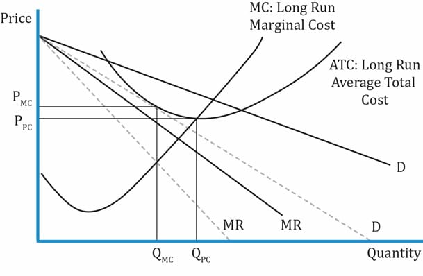
Interpretation of the graph:
- The solid lines show the original demand and MR curves.
- The dashed lines show the shift in the demand and MR curves when a new firm enters the market.
- Short-run economic profits of existing firms encourage new firms to enter the market as the barriers to entry are low. When new firms enter, the demand curve shifts to the left and the market share of existing firms falls. The number of products in the market increases.
- In the long run, firms will enter and exit until P = ATC. At this point, economic profit will be zero and there will no longer be an incentive for new firms to enter the market. Therefore, long-run equilibrium is established.
- QMC and PMC are the equilibrium quantity and price respectively, for monopolistic competition. QPC and PPC are the equilibrium quantity and price respectively, for perfect competition. As you can see, the equilibrium price is higher and the quantity is lower for monopolistic competition.
The table below summarizes the similarities and differences between perfect competition and monopolistic competition.
| Perfect Competition (PC) vs. Monopolistic Competition (MC) |
| Similarities |
Ways in which MC is different from PC. |
| Long-run economic profit is zero |
In the long run, profit-maximizing output quantity of MC is lower than PC. |
| Profit-maximizing output: MR = MC |
Economic cost in MC includes advertising cost for product differentiation. |
|
PC is efficient as surplus is maximized.
PC: Price = Marginal Cost
MC: Price > Marginal Cost
Deadweight loss in MC because firms have some amount of pricing power and consumer surplus is lost. |
|
Prices are lower in PC, but consumers have little variety. |
Share on :


 Do IFT Mocks to make you exam-ready!


