LM01 Topics in Demand and Supply Analysis

Part 4

12. Economies and Diseconomies of Scale with Short-Run and Long-Run Cost Analysis

Economists use two time horizons based on how firms are able to vary the quantity of input: short run and long run. In the short run, at least one of the inputs or factors of production is constant. In the long run, all factors of production are variable.

Short- and Long-Run Cost Curves

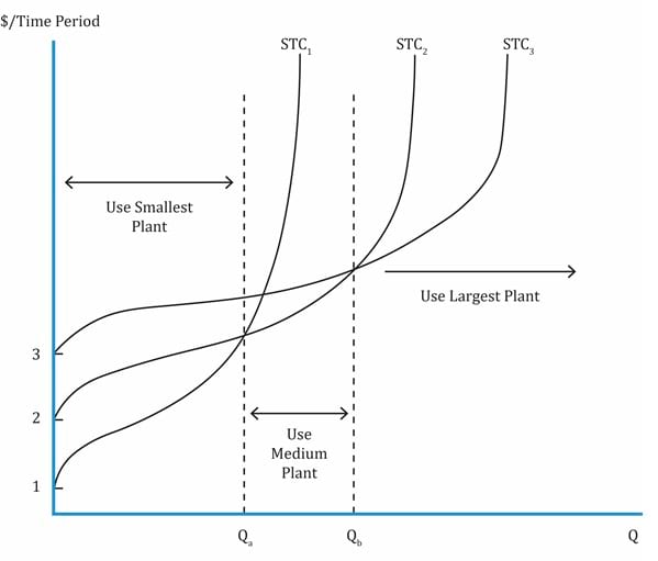
The graph below shows a set of short-run total cost curves for each level of capital input.

In the long run:

• All factors of production (both labor and capital) are variable.
• Think of the long-run total cost curve (LTC) as a combination of several STCs. By drawing a tangent to the minimum point of all the SRATC curves and connecting them, we get the LTC curve for the firm.
• The LTC is called the envelope curve. It envelops or encompasses all combinations of technology, plant size, and physical capital.

Defining Economies of Scale and Diseconomies of Scale

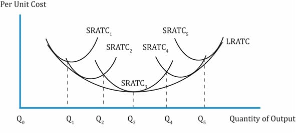
Each STC curve has a corresponding short-run average total cost curve (SRATC). The STCs for different plant sizes and the corresponding long-run average total cost curve (LRATC) is shown in the exhibit below.

Interpretation of the graph:

• The SRATC defines what the per-unit cost will be for any quantity in the short run.
• The SRATC shifts down and to the right. Note that as plant size increases, the per-unit cost decreases as can be seen in the case of SRATC
• The LRATC is derived from connecting the lowest level of STC for each level of output.
• The shape of the long-run cost curve depends on whether the firm is facing economies of scale or diseconomies of scale.
• Economies of scale is the decrease in the long-run cost per unit as output increases. LRATC has a negative slope when there are economies of scale. The portion to the left of Q₃ represents economies of scale.
• Q₃ represents the minimum efficient scale. It is the output level at which the long-run average total cost is the lowest and the output is optimal. This portion exhibits constant returns to scale where long-run average total costs do not change as output quantity increases.
• Beyond Q₃, the LRATC goes up. This portion represents diseconomies of scale. Here there is an increase in long-run cost per unit as output increases. LRATC has a positive slope when there are diseconomies of scale. The right side of LRATC curve represents diseconomies of scale.

The factors contributing to economies of scale and a lower ATC are as follows:

• Increasing returns to scale: increase in output is relatively larger than the increase in input. The left side of Q₃ shows increasing returns to scale.
• Division of labor/management.
• Technologically/economically efficient equipment that results in increased productivity.
• Effective decision-making.
• Reduce waste and lowering costs through better quality control.
• Bulk purchases resulting in lower prices.

The factors contributing to diseconomies of scale are as follows:

• Decreasing returns to scale: Increase in output is relatively less than the increase in input. The right side of Q₃ shows decreasing returns to scale.
• Higher resource costs due to supply bottlenecks.
• Improper management because of size.
• Duplication of product lines.
• Higher labor costs.

Share on :