LM01 Topics in Demand and Supply Analysis

Part 3

7.  Supply Analysis: Cost, Marginal Return, and Productivity

Marginal Returns and Productivity

Factors of production are the inputs used by a firm to produce goods and services. These inputs include land, labor, capital, and raw materials. For simplicity, we will consider only two inputs:

• Labor (L): skilled, unskilled, management personnel, etc.
• Capital (K): physical capital such as machinery, equipment, and tools used by labor to produce output.

Before moving on, let us understand a few basic terms.

• Marginal product of labor: Increase in the quantity of output from an additional unit of labor.
• Marginal product of capital: Increase in the quantity of output from an additional unit of capital.
• Productivity: Average output per unit of input (such as labor or capital).
• Increasing marginal returns: Increase in productivity as the quantity of an input increases.
• Law of diminishing marginal returns: As more and more units of an input resource are added, productivity will eventually decrease.

Cost of production. The total cost of production is given by the equation below:

where:

w is the wage rate per hour

L is the number of labor hours

r is the cost per hour of capital and

K is number of hours for which capital is used.

Two factors that lower the cost of producing at a given level of output are:

• Increase in input productivity.
• Decrease in input prices.

Total Product, Average Product, and Marginal Product

Total product is the total output from all inputs during a time-period. It is denoted by TP or Q. Total product gives information about the total production of a firm during a time-period, but reveals very little about how efficient the firm is.

Average product is the total product divided by the quantity of a given input.  It measures the productivity of an input. The average product of labor is given by: or .

Marginal product is the amount of additional output resulting from using one more unit of input, assuming other inputs are fixed. It is calculated by dividing the change in total product by the change in the quantity of input. Hence, the marginal product of labor is: or

Let us take an example of three companies X, Y and Z whose total product and average product of labor are given below:

It is not possible to identify the most efficient company by looking at just the TP values. AP is a better measure of efficiency. Company X has the highest AP and is therefore the most efficient.

The table below shows TP, AP and MP of labor for a firm across different levels of labor:

Interpretation:

• The total product (output) increases till the sixth unit of labor and declines when the seventh unit of labor is added. Hence the total product is maximum (420) with 6 units of labor.
• When we go from one unit of labor to two units of labor the marginal product (MP) increases. This implies increasing marginal returns. The marginal product for the second unit of labor is calculated as: 
• When a third unit of labor is added the MP decreases. This implies diminishing marginal returns.

Breakeven and Shutdown Analysis

7. Economic Profit Versus Accounting Profit

Economic profit is the difference between the total revenue and total economic costs. It is also known as abnormal profit. Another definition of profit is accounting profit. Accounting profit is the difference between the total revenue and total accounting costs.

Economic profit = Total revenue – Total economic costs

Economic profit = Accounting profit – Total implicit opportunity costs

Accounting profit = Total revenue – Total accounting costs

Economic cost considers opportunity costs, while accounting cost does not. Economic cost is the sum of accounting cost and opportunity cost. Let us take an example. Assume Megan starts a business with an equity capital of $100 million. The required return on the invested amount is 10%.  Hence, the opportunity cost is 10% of $100 million = $10 million. If the accounting cost is $190 million, then the total economic cost is $200 million. Continuing with this example, if the revenue is $200 million, the economic profit is zero and the accounting profit is $10 million. In this case, it can be said that the business is earning a normal profit of $10 million.

Instructor’s Note:

In this reading, ‘cost’ refers to economic cost and ‘profit’ refers to ‘economic profit’.

If a firm’s revenue is equal to the firm’s total economic cost, the economic profit is zero and the firm is said to be earning a normal profit.

Accounting profit = economic profit + normal profit.

Normal profit = implicit costs or opportunity costs.

9. Marginal Revenue, Marginal Cost and Profit Maximization; Short-Run Cost Curves: Total, Variable, Fixed, And Marginal Costs

Marginal Revenue

Marginal revenue is defined as the change in total revenue divided by the change in quantity. It is the incremental revenue because of producing an additional unit per time-period. It is expressed as:

We will now analyze marginal revenue under two market conditions: perfect competition and imperfect competition.

Marginal revenue under perfect competition

In a perfectly competitive market:

• There are many buyers and sellers and the interaction between them determines the equilibrium price.
• All the firms are relatively small and the products sold by the firms are identical, or homogeneous.
• All the firms are price takers. They have no pricing power – that is, the individual consumers and sellers cannot influence the market price of a good/service in any way.
• Any quantity of the product can be sold at the market price. But, a small increase in price would mean losing all sales. Example: wheat.
• The demand curve is horizontal or perfectly elastic.
• In a perfectly competitive market, MR = AR = P. Price is constant. This implies that total revenue increases by P if the quantity increases by one unit.

Marginal revenue under imperfect competition

In an imperfect competitive market:

• The firms sell differentiated products and have a large market share.
• There may not be any close substitutes.
• Marginal revenue intersects the x-axis at the point where total revenue is maximized.
• The marginal revenue and demand curve are downward sloping.

Marginal Cost

Marginal cost is the incremental cost of producing one more unit.  It can be calculated by dividing the change in total cost by the change in quantity. It is expressed as:

Economists distinguish between short-run and long-run marginal cost. Short-run marginal cost is the cost of producing an additional unit assuming only labor costs vary and all other factors of production are constant. Short-run marginal cost is directly related to wage price and inversely related to productivity. Short-run marginal cost, . Long-run marginal cost is the cost of producing one more unit assuming all factors of production are variable.

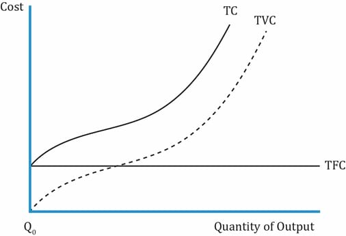
Fixed and Variable Costs

Total cost can be broken down into fixed and variable costs. Fixed costs do not change with the quantity of output.  Variable costs change with the quantity of output. Average variable cost is the ratio of total variable cost to quantity. It is expressed as:

Profit Maximization

A firm’s profit is maximized at a level of output where marginal revenue is equal to marginal cost (MR = MC).  If marginal revenue exceeds marginal cost, a firm can increase profits by producing more. If marginal revenue is less than marginal cost, the firm should scale back.  This discussion assumes that marginal cost is rising with increased output.

Understanding the Interaction between Total, Variable, Fixed, and Marginal Cost and Output

All the graphs we look at in this section are from a short-run perspective. In the short run, one or more factors of production are fixed. Usually capital is fixed in the short run while labor may change. The graph below shows the cost curves for a firm in the short run.

Interpretation of the graph:

• Total fixed cost is constant or flat for any given output level. It does not change as production varies.
• Total variable cost increases as the quantity of output increases. For simplicity, it is assumed to have a linear relationship with quantity. If there is no production, then TVC is zero.
• The total cost for any quantity of output is the sum of total fixed cost and total variable cost. It also increases as production increases and the quantity of output increases.

The graph below shows the MC, ATC and AVC curves for a firm in the short run.

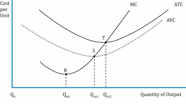
Interpretation of the graph:

AVC Curve

• The AVC curve is U-shaped but this can vary from company to company, or industry to industry.
• As output increases, average variable cost falls to a minimum and then increases. It falls, because the total fixed cost is distributed over a large number of units.

ATC Curve

• Like the AVC curve, the ATC curve is also U-shaped but higher than the AVC curve because:
  • AFC is added to AVC for any given quantity of output.
  • AVC increases more quickly than AFC decreases.
• The distance between the ATC and AVC for any output quantity will be AFC.

Marginal cost curve

• MC intersects AVC at its lowest point, S. The corresponding quantity is . MC is greater than AVC beyond
• If the marginal cost of producing one more unit is less than the average variable cost (to the left of the minimum point), then it will pull the AVC down.
• Similarly, if the marginal cost of producing one more unit is greater than the average variable cost (to the right of the minimum AVC point), then it will pull the AVC up.
• The lowest point for the ATC is T, where MC equals ATC. Beyond T, MC is greater than ATC.

AFC

• The difference between ATC and AVC for any quantity will be AFC. AFC is also the total fixed cost divided by the quantity.
• Average fixed cost falls as output increases because the numerator in the above formula is constant while the denominator increases. Put differently, the total fixed cost is spread over a larger output, so it slopes downward as output quantity increases.

10. Perfect and Imperfect Competition, Profit Maximization

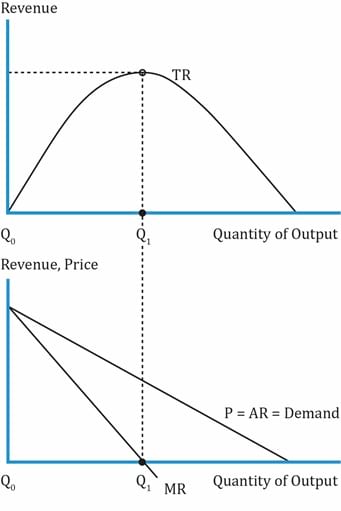
Revenue under Conditions of Perfect and Imperfect Competition

Total revenue under perfect competition:

• Total revenue is the price multiplied by quantity (TR = P x Q).
• The firm has no pricing power, and price is decided by the market.
• The demand curve is horizontal and slope is zero.
• Market price is equal to marginal revenue, which is equal to average revenue. P = MR = AR.
• TR increases by the price for every incremental increase in output. The TR curve is linear and positively sloped.

Total revenue under imperfect competition

• The firm has a large market share.
• The demand curve is downward sloping. The firm must decrease the price in order to sell more.
• Total revenue increases with greater quantity. However, there is a quantity at which the profit is maximized. Beyond this, any price decrease will result in a decrease in total revenue as the effect of the decrease in price will be greater than the quantity sold.
• The TR curve for such a firm is initially zero, then it increases and subsequently decreases. It increases when MR is positive and demand is elastic. It falls when MR is negative and demand is inelastic. TR is maximum when MR is zero.

Profit Maximization, Breakeven, and Shutdown Points of Production

Profit is maximized when:

• Marginal revenue equals marginal cost. MR = MC.
• MC is rising.
• Alternatively, when the difference between total revenue and total cost is the greatest.

The graph below shows the TR, TC, demand curve, and profit maximization under perfect competition.

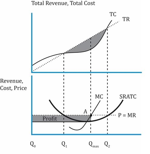
Q_max is the profit maximizing quantity where MR = MC and MC is rising.

11. Break Even Analysis and Shutdown Decision

Breakeven Analysis

A firm is said to breakeven under the following conditions:

• total revenue equals total costs (TR = TC).
• price (average revenue) equals average total costs (AR = ATC).

When a firm is operating at its breakeven point, the economic profit is zero.  It might still be earning a positive accounting profit.

A perfectly competitive market with no barriers to entry will attract new entrants. The increased competition will lead to increased output and lower prices in the long run where no firm is able to earn an excess return or positive economic profit.

Instructor’s Note

If economic profit is zero, accounting profit is called normal profit.

Under perfect competition, firms earn only normal profits in the long run.

The Shutdown Decision

The relationships that show when a firm must operate or shutdown are given in the table below:

Let us understand a firm’s breakeven and shutdown point using the graph below.

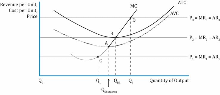
Interpretation of the graph:

• Assume the price at P₃ is 150. If the competition is perfect, then P₃ is the demand curve and MR = AR.
• At any point on the MC between P₂ and P₃, the firm is profitable because the average revenue is greater than the average total cost.
• The breakeven point is the point where P = ATC = MC. Graphically, it is the point where MC intersects ATC. The corresponding quantity is the breakeven quantity, . Suppose this price is 100.
• Between A and B, the price is greater than AVC. The firm will continue to operate in the short run even though it is not profitable.
• To the left of A, the price is less than AVC. The firm will shut down.

Share on :