LM02 The Firm and Market Structures

Part 3

10. Oligopoly & Demand Analysis and Pricing Strategies in Oligopoly Markets: Pricing Independence Portion

An oligopoly market has few sellers of a product and many buyers. These sellers are large players in their industry who determine the prices or quantities. For example, credit card companies such as Visa, MasterCard, and Amex.

Characteristics:

• There are a small number of potential sellers.
• The products offered by each seller are close substitutes for the products offered by the other firms and may be differentiated by brand or be homogeneous and unbranded.
• Entry into the market is difficult with fairly high costs and significant barriers to competition.
• Firms typically have substantial pricing power. Since there are very few firms, the pricing decisions are interdependent. Whenever a firm makes a decision, it must take into account how the competing firms will react.
• Products are often highly differentiated through marketing, features, and other non-price strategies.
• The pricing is strategic and firms in an oligopoly have a temptation to collude.

10.1. Demand Analysis and Pricing Strategies in Oligopoly Markets

If firms collude, the total market demand is divided among the individual participants. The firms act like a cartel and decide how to divide the demand, and what price to set for the products in order to maximize profit.

If firms do not collude, each firm faces an individual demand curve and a market demand curve. There are several models that try to explain pricing in oligopoly markets:

• Pricing interdependence
• Cournot assumption
• Nash equilibrium
• Stackelberg model

Pricing Interdependence – Kink Demand Curve

According to this theory, a competitor will not follow a price increase, but will cut prices in response to a price decrease.

Example: Let us assume a town has two cola suppliers: Coke and Pepsi. This type of oligopoly is called a duopoly. Now, assume the initial equilibrium price of 1 liter Coke bottle is 100 and the quantity is 5000.

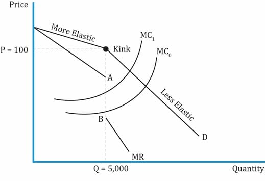
Effect of price increase: If Coke increases its price from 100 to 105, what will Pepsi do? According to the interdependence theory, Pepsi will not increase the price and consumers will switch from Coke to Pepsi. The quantity demanded of Coke will decrease (see the elastic portion of the demand curve).

Effect of price decrease: Instead, if Coke decreases the price to 95, then Pepsi will also decrease the price to 95. The quantity demanded of Coke will increase when the price decreases, but not by much because there is no substitution effect. Consumers do not switch from Pepsi to Coke as both are selling at the same price. To the right of the kink, the demand curve is inelastic.

Some important points:

• There are two different demand curves in the model; combining them gives us the overall demand, which is a kinked (bent) curve. A kink in the demand curve leads to a discontinuous (with a gap) marginal revenue curve. One part of the MR curve corresponds to the price increase part of the demand curve and the other to the price decrease part of the demand curve.
• Profit-maximizing rule: MR = MC.
• Equilibrium price and quantity do not change so long as the marginal-cost curve of the firm falls between the gaps in the MR curve.
• The MC must change considerably for the firms to change their price.
• Advantage: The model helps explain stable prices.
• Disadvantage: It does not tell us what the prices should be.

11. Oligopoly & Demand Analysis and Pricing Strategies in Oligopoly Markets: The Cournot Assumption Part

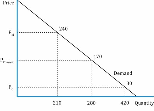
Cournot Assumption

Firms compete simultaneously to determine a profit-maximizing output, based on the assumption that the other firms’ output will not change.  In the long run, change in price or quantity will NOT increase profits. As the number of firms in an oligopoly increase, the equilibrium point moves closer to perfect competition.

Assume there are two firms with the output levels q₁ and q₂ respectively. Firm 1 chooses its output as q₁ to maximize profit based on the assumption that firm 2’s output level q₂ is constant in the future. Similarly, firm 2 chooses its output as q₂ to maximize profits by assuming that firm 1’s output level is constant. Firms choose q₁ and q₂ simultaneously. Let us now look at the price and quantity numbers associated with the Cournot assumption.

• With a monopoly, the price is highest and quantity is lowest.
• In a perfect competition market structure, the price is lowest and quantity is highest.
• In a duopoly market characterized by the Cournot assumption, both the price and quantity will lie somewhere in between. As the number of firms increase, the equilibrium point moves towards perfect competition.

12. Oligopoly & Demand Analysis and Pricing Strategies in Oligopoly Markets: The Nash Equilibrium part

The Nash Equilibrium in a Duopoly Market

Unlike perfect competition, in oligopoly there is a lot of strategic interdependence between firms. Since the number of firms are few, the actions one takes affects the others.

Nash Equilibrium: A set of choices/strategies among two or more participants is called a Nash equilibrium if, holding the strategies of all other participants constant, no participant has an incentive to choose a different strategy. In an oligopoly, firms arrive at an equilibrium strategy after considering the actions of other firms (interdependence). Once they arrive at equilibrium, no firm wants to change its strategy.

Assumptions made in Nash equilibrium:

• The firms do the best they can, given the actions of their rivals.
• The actions are interdependent.
• The firms do not cooperate (collude); each firm wants to maximize its own profits.

Example: WesCo and RifCo sell a similar product. Each company can employ a high-price strategy or a low-price strategy. The profit for each strategy is shown. What is the Nash equilibrium?

The four possible strategies are shown in the four boxes. For example, box 1 on the top-left corner has WesCo adopting a low price strategy and RifCo adopting a low price strategy as well. The profit for WesCo is 50 and that for RifCo it is 70. At any point in time, the companies can be in only one box. It is not possible for WesCo to adopt a low price strategy with profit of 50 (box 1) and RifCo to adopt a high price strategy with profit of 0 (box 2).

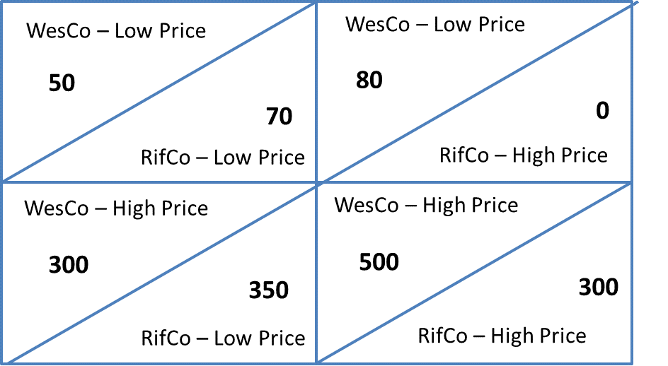
No matter where the companies start, they will end up in box 4 (lower left box).

Let’s start with box 1. The total profit of WesCo and RifCo is 120. They are both selling the products at a lower price. It is in WesCo’s best interest to increase prices, and their profits jump from 50 to 300 in box 4. It is in RifCo’s best interest as well if WesCo increases the price, as RifCo can also increase the price. RifCo’s profit jumps from 70 to 350. The combined profit of box 4 now is 650.

The combined profits are the highest in box 3, which is 800. Both the companies are charging high prices. Box 3 is in WesCo’s best interest as it earns its maximum profit of 500, but it’s possible only if RifCo also charges the high price. But RifCo is not happy here and would lower the prices to increase its profit from 300 (box 3) to 350 (box 4).

When RifCo lowers its price to make a profit of 350 in box 4, WesCo’s profit falls from 500 to 300. The Nash equilibrium position in box 4 is what they arrive at finally.

Can both companies be better if they collude? Yes, if both the companies agree to collude and charge high prices. If WesCo and RifCo agree to split the maximum profit of 800 equally, then each company makes a profit of 400, which is better than the Nash equilibrium profit of 300 and 350 profit respectively. Companies are said to form a cartel when they engage in collusive agreements openly.

Factors that affect the chances of successful collusion:

1. Number and size of sellers: The number of firms should be small.
2. Similarity of products: Products must be homogeneous.
3. Cost structure: Firms must have a similar cost structure.
4. Order size and frequency: Orders must be small and frequent.
5. Retaliation: Threat from competitors is weak.
6. Degree of external competition: High external competition.

Stackelberg Model

There is one dominant large firm and many small firms. The large firm sets the price and has the first mover advantage.

In the Stackelberg model, the decision-making happens sequentially (recall it happens simultaneously in the Cournot assumption). The leader firm chooses the output first and then the follower firm chooses its output.

13. Supply Analysis & Optimal Price and Output & Long-Run Equilibrium in Oligopoly Markets

The curriculum discusses the supply analysis for only one type of oligopoly – the dominant firm oligopoly.

• As in monopolistic competition, the supply function is not well defined.
• We cannot determine equilibrium output and price without considering the demand function and competitive strategies.
• Profit-maximizing condition: MR = MC.
• The equilibrium price is based on the demand curve.

Example: Say we have an oligopoly market where one firm has a significantly lower cost of production than its competitors and has a 40% market share. A dominant or leader firm is a firm with at least 40 % market share, greater capacity, lower cost structure, and is price maker. A follower firm is a small firm that is a price taker – i.e. it accepts the price set by the leader firm. Let us say there are five such firms in this market.

The graph below shows the quantity that will be supplied and the price charged by the market leader, as well as by the other firms.

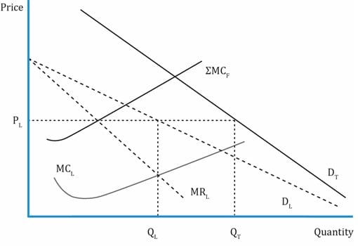
Interpretation of the graph:

• Price is plotted on the y-axis and quantity on the x-axis.
• The solid line represents an aggregate market demand. The following are the curves for the dominant firm:
  • Dashed line – the demand curve.
  • MR_L – the marginal revenue curve; it lies below the demand curve and is steeper
  • MC_L – the marginal cost curve.
  • P_L – optimal price.
• Assuming the other five firms will take the price established by the leader, the overall market demand is given as Q_T. The small/follower firms have no incentive to slash prices as it will lead to price wars with the leader, who is a low-cost producer.
• Quantity supplied by the leader firm = Q_L; quantity supplied by the other firms = Q_T­ – Q_L.
• Notice that the demand curves of the industry and of the dominant firm are not parallel to each other. As the price decreases, the difference between the curves diminishes. The reasons are:
  • The dominant firm is a low cost producer. When prices start falling, the other smaller firms exit the industry because they do not want to sell below cost.
  • The dominant firm gets a greater market share as other firms exit, and Q_L (quantity supplied by the leader) increases.

13.1 Optimal Price and Output in Oligopoly Markets

There is no single optimum price and output model that works for all oligopoly market situations because of different strategies and pricing methods. The process for determining the optimal price for a few methods is listed below:

• Kinked demand curve: Price at the kink in demand function.
• Dominant firm: Price at the quantity where MR = MC. Followers take the leader’s price.
• Cournot assumption: No changes in price and output by other firms once the dominant firm chooses its output level where MR=MC.
• Nash equilibrium: Each firm acts in its best interest under the given circumstances. No certainty of price and output level.

13.2. Factors Affecting Long-Run Equilibrium in Oligopoly Markets

Long-run economic profits are possible, but empirical evidence suggests that over time the market share of the dominant firm declines.

Share on :