
This reading covers:
The market is defined as a group of buyers and sellers that are aware of each other, and are able to agree on a price for the exchange of goods and services.
The market structure is classified into the following four categories:
Perfect competition and monopoly are two extremes of the market structure in terms of number of firms and profits with the other types falling somewhere in between.
The five factors that determine market structure are:
The table below summarizes the basic characteristics of the four market structures:
| Perfect Competition | Monopolistic Competition | Oligopoly | Monopoly | |
| Number of Sellers | Many firms | Many firms | Few firms | Single firm |
| Barriers to Entry and Exit | Very low | Low | High | Very high |
| Product Differentiation | Homogeneous | Substitutes but differentiated | Close substitutes or differentiated | Unique product |
| Non-price Competition | None | Advertising and product differentiation | Advertising and product differentiation | Advertising |
| Pricing Power | None. Price taker. | Some | Some to significant | Considerable |
| Example | Oranges; Milk; Wheat | Toothpaste | Prices of commercial airlines for a given route | Electricity provider/any utility company (water, cooking gas) as they are typically controlled by a government authority |
Note: This table is important from an exam perspective.
The most preferred market structure by producers is monopoly/oligopoly because they offer the highest pricing power. The most preferred market structure by consumers is perfect competition as prices are lower.
The characteristics of perfect competition are as follows:
The graph below shows the market demand curve for a perfectly competitive market. Here price is plotted on the y-axis and quantity on the x-axis and the market demand curve is downward sloping:
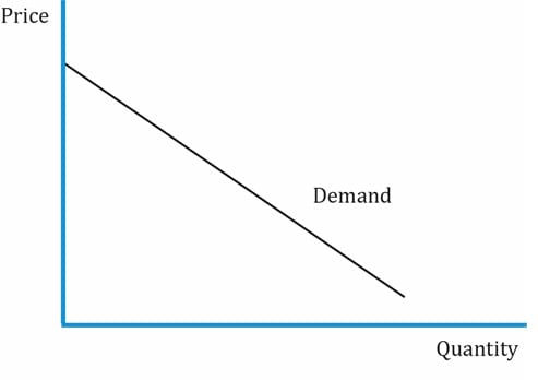
To understand this curve, let’s assume that the market demand is given by the following equation:
Q = 50 – 2P where Q = quantity demanded and P = product’s price.
Rearranging, we get P = 25 – 0.5Q
Total revenue: TR = P * Q = 25 Q – 0.5Q2

(Using calculus, the first derivative of 0.5 * Q2 is 2 * 0.5 * Q = Q)
We derived this based on two assumptions which are often not true in the real world:
Movement along the demand curve happens only if the price and quantity demanded of the product changes, all else constant. If any factor other than price/quantity demanded changes, then there is a shift in the demand curve. For instance, an increase in income will cause the demand curve to shift up.
Price elasticity of demand measures the sensitivity of quantity demanded to a change in price. It depends on the following three factors:
| Factors affecting price elasticity of demand | |
| Substitutes | Elasticity is high if there are more close substitutes i.e. customers are more sensitive to price changes. If the price of a substitute goes down, the quantity demanded of the substitute goes up and the quantity demanded of the original product goes down. |
| The share of the consumer’s budget spent on the item | The greater the share, the higher the price elasticity.
Ex: Expensive goods such as cars are highly elastic. Grocery essentials such as cereals, sugar and salt are inelastic. A 10% increase in the price of cars and cereals will affect the demand for cars but not that of cereals. |
| Length of time within which demand schedule is being considered | The longer the period, the higher the elasticity.
Ex: If the price of cooking gas increases, the demand will not change much in the short run; however, demand will decline in the long run as consumers switch to electric stoves. |
Numerically, price elasticity of demand falls into three categories:
| Price elasticity of demand | |
| Elastic demand | |ε| > 1; a 1% change in price will cause a more than 1% change in quantity demanded. Ex: furniture (ε = 3.15). |
| Unitary elastic demand | |ε| = 1 |
| Inelastic demand | |ε| < 1; a 1% change in price will cause a less than 1% change in quantity demanded. Ex: coffee (ε = 0.16). |
| Special Cases | |
| Perfectly elastic or horizontal demand schedule | Horizontal demand curve. At a given price, quantity demanded is infinite. ε = ∞. Ex: corn. |
| Perfectly inelastic or vertical demand schedule | Vertical demand curve. Quantity demanded is fixed irrespective of price. ε = 0. Ex: insulin. |
Income elasticity of demand is the percentage change in the quantity demanded, divided by a percentage change in income, all else equal. It measures how sensitive the quantity demanded is to changes in income.
Cross-price elasticity of demand measures how the quantity demanded of a good changes when there is a change in the price of another good.
Instructor’s Note: Changes in own price causes a movement along the demand curve, whereas, changes in income and price of substitutes cause a shift in the demand curve.
Consumer surplus is the difference between the price that consumers are willing to pay (value) and the price that they actually pay (expenditure).
On a supply and demand curve, it is the area beneath the demand curve and above the price paid.
The total consumer surplus received from buying Q1 units at a level price of P1 per unit is the difference between the area under the demand curve and the area of the rectangle P1 × Q1. This is represented by the triangle.
Example:
(This is based on Example 1 from the curriculum.)
A market demand function is given by the equation QD = 180 – 2P. Find the value of consumer surplus if price is equal to 65.
Solution:
Quantity demanded at the price of 65 is: QD = 180 – 2(65) = 50
The inverted demand function is: P = 90 – 0.5QD
Using this information, we can draw the following demand curve.
Consumer surplus = area of the triangle in the upper section = ½ (Base)(Height) = ½ (50)(25) = 625


Ace the Exam with Active Learning!

Ace the Exam with IFT Notes!
 Do IFT Mocks to make you exam-ready!

Practice your way to success!

Accelerate your studies!


Sign up to get more!